Analyzing your Results
Several nbodykit algorithms compute binned clustering statistics
and store the results as a BinnedStatistic object (see a list
of these algorithms here. In this section,
we provide an overview of some of the functionality of this class to help
users better analyze their algorithm results.
The BinnedStatistic class is designed to hold data variables at
fixed coordinates, i.e., a grid of \((r, \mu)\) or \((k, \mu)\) bins
and is modeled after the syntax of the xarray.Dataset object.
Loading and Saving Results
A BinnedStatistic object is serialized to disk using a
JSON format. The to_json() and
from_json() functions can be used to save and load
BinnedStatistic objects. respectively.
To start, we read two BinnedStatistic results from JSON files,
one holding 1D power measurement \(P(k)\) and one holding a 2D power
measurement \(P(k,\mu)\).
[2]:
from nbodykit.binned_statistic import BinnedStatistic

data_dir = os.path.join(os.path.abspath('.'), 'data')
power_1d = BinnedStatistic.from_json(os.path.join(data_dir, 'dataset_1d.json'))
power_2d = BinnedStatistic.from_json(os.path.join(data_dir, 'dataset_2d.json'))
Coordinate Grid
The clustering statistics are measured for fixed bins, and the
BinnedStatistic class has several attributes to access the
coordinate grid defined by these bins:
shape: the shape of the coordinate griddims: the names of each dimension of the coordinate gridcoords: a dictionary that gives the center bin values for each dimension of the gridedges: a dictionary giving the edges of the bins for each coordinate dimension
[3]:
print("1D shape = ", power_1d.shape)
print("2D shape = ", power_2d.shape)
1D shape =  (64,)
2D shape =  (64, 5)
[4]:
print("1D dims = ", power_1d.dims)
print("2D dims = ", power_2d.dims)
1D dims =  ['k']
2D dims =  ['k', 'mu']
[5]:
print("2D edges = ", power_2d.coords)
2D edges =  {'k': array([0.00613593, 0.01840777, 0.03067962, 0.04295147, 0.05522331,
       0.06749516, 0.079767  , 0.09203884, 0.10431069, 0.11658255,
       0.1288544 , 0.14112625, 0.1533981 , 0.1656699 , 0.17794175,
       0.1902136 , 0.20248545, 0.2147573 , 0.22702915, 0.239301  ,
       0.25157285, 0.2638447 , 0.27611655, 0.2883884 , 0.30066025,
       0.3129321 , 0.32520395, 0.3374758 , 0.3497476 , 0.36201945,
       0.3742913 , 0.38656315, 0.398835  , 0.41110685, 0.4233787 ,
       0.43565055, 0.4479224 , 0.46019425, 0.4724661 , 0.48473795,
       0.4970098 , 0.5092816 , 0.52155345, 0.5338253 , 0.54609715,
       0.558369  , 0.57064085, 0.5829127 , 0.59518455, 0.6074564 ,
       0.61972825, 0.6320001 , 0.64427195, 0.6565438 , 0.6688156 ,
       0.68108745, 0.6933593 , 0.70563115, 0.717903  , 0.73017485,
       0.7424467 , 0.75471855, 0.7669904 , 0.77926225]), 'mu': array([0.1, 0.3, 0.5, 0.7, 0.9])}
[6]:
print("2D edges = ", power_2d.edges)
2D edges =  {'k': array([0.        , 0.01227185, 0.02454369, 0.03681554, 0.04908739,
       0.06135923, 0.07363108, 0.08590292, 0.09817477, 0.1104466 ,
       0.1227185 , 0.1349903 , 0.1472622 , 0.159534  , 0.1718058 ,
       0.1840777 , 0.1963495 , 0.2086214 , 0.2208932 , 0.2331651 ,
       0.2454369 , 0.2577088 , 0.2699806 , 0.2822525 , 0.2945243 ,
       0.3067962 , 0.319068  , 0.3313399 , 0.3436117 , 0.3558835 ,
       0.3681554 , 0.3804272 , 0.3926991 , 0.4049709 , 0.4172428 ,
       0.4295146 , 0.4417865 , 0.4540583 , 0.4663302 , 0.478602  ,
       0.4908739 , 0.5031457 , 0.5154175 , 0.5276894 , 0.5399612 ,
       0.5522331 , 0.5645049 , 0.5767768 , 0.5890486 , 0.6013205 ,
       0.6135923 , 0.6258642 , 0.638136  , 0.6504079 , 0.6626797 ,
       0.6749515 , 0.6872234 , 0.6994952 , 0.7117671 , 0.7240389 ,
       0.7363108 , 0.7485826 , 0.7608545 , 0.7731263 , 0.7853982 ]), 'mu': array([0. , 0.2, 0.4, 0.6, 0.8, 1. ])}
Accessing the Data
The names of data variables stored in a BinnedStatistic are stored in
the variables attribute, and the data attribute stores the
arrays for each of these names in a structured array. The data for a given
variable can be accessed in a dict-like fashion:
[7]:
print("1D variables = ", power_1d.variables)
print("2D variables = ", power_2d.variables)
1D variables =  ['power', 'k', 'mu', 'modes']
2D variables =  ['power', 'k', 'mu', 'modes']
[8]:
# the real component of the 1D power
Pk = power_1d['power'].real
print(type(Pk), Pk.shape, Pk.dtype)

# complex power array
Pkmu = power_2d['power']
print(type(Pkmu), Pkmu.shape, Pkmu.dtype)
<class 'numpy.ndarray'> (64,) float64
<class 'numpy.ndarray'> (64, 5) complex128
In some cases, the variable value for a given bin will be missing or invalid,
which is indicated by a numpy.nan value in the data array for
the given bin. The BinnedStatistic class carries a mask
attribute that defines which elements of the data array have
numpy.nan values.
Meta-data
An OrderedDict of meta-data for a
BinnedStatistic class is stored in the attrs attribute.
Typically in nbodykit, the attrs dictionary stores
information about box size, number of objects, etc:
[9]:
print("attrs = ", power_2d.attrs)
attrs = {'N1': 4033, 'Lx': 512.0, 'Lz': 512.0, 'N2': 4033, 'Ly': 512.0, 'volume': 134217728.0}
To attach additional meta-data to a BinnedStatistic class, the user
can add additional keywords to the attrs dictionary.
Slicing
Slices of the coordinate grid of a BinnedStatistic can be achieved
using array-like indexing of the main BinnedStatistic object, which
will return a new BinnedStatistic holding the sliced data:
[10]:
# select the first mu bin
print(power_2d[:,0])
<BinnedStatistic: dims: (k: 64), variables: ('power', 'k', 'mu', 'modes')>
[11]:
# select the first and last mu bins
print(power_2d[:, [0, -1]])
<BinnedStatistic: dims: (k: 64, mu: 2), variables: ('power', 'k', 'mu', 'modes')>
[12]:
# select the first 5 k bins
print(power_1d[:5])
<BinnedStatistic: dims: (k: 5), variables: ('power', 'k', 'mu', 'modes')>
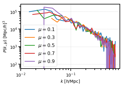
A typical usage of array-like indexing is to loop over the mu dimension
of a 2D BinnedStatistic, such as when plotting:
[13]:
from matplotlib import pyplot as plt

# the shot noise is volume / number of objects
shot_noise = power_2d.attrs['volume'] / power_2d.attrs['N1']

# plot each mu bin separately
for i in range(power_2d.shape[1]):
    pk = power_2d[:,i]
    label = r"$\mu = %.1f$" % power_2d.coords['mu'][i]
    plt.loglog(pk['k'], pk['power'].real - shot_noise, label=label)

plt.legend()
plt.xlabel(r"$k$ [$h$/Mpc]", fontsize=14)
plt.ylabel(r"$P(k,\mu)$ $[\mathrm{Mpc}/h]^3$", fontsize=14)
plt.show()
The coordinate grid can also be sliced using label-based indexing, similar to
the syntax of xarray.Dataset.sel(). The method keyword of
sel() determines if exact
coordinate matching is required (method=None, the default) or if the
nearest grid coordinate should be selected automatically (method='nearest').
For example, we can slice power spectrum results based on the
k and mu coordinate values:
[14]:
# get all mu bins for the k bin closest to k=0.1
print(power_2d.sel(k=0.1, method='nearest'))
<BinnedStatistic: dims: (mu: 5), variables: ('power', 'k', 'mu', 'modes')>
[15]:
# slice from k=0.01-0.1 for mu = 0.5
print(power_2d.sel(k=slice(0.01, 0.1), mu=0.5, method='nearest'))
<BinnedStatistic: dims: (k: 8), variables: ('power', 'k', 'mu', 'modes')>
We also provide a squeeze() function which behaves
similar to the numpy.squeeze() function:
[16]:
# get all mu bins for the k bin closest to k=0.1, but keep k dimension
sliced = power_2d.sel(k=[0.1], method='nearest')
print(sliced)
<BinnedStatistic: dims: (k: 1, mu: 5), variables: ('power', 'k', 'mu', 'modes')>
[17]:
# and then squeeze to remove the k dimension
print(sliced.squeeze())
<BinnedStatistic: dims: (mu: 5), variables: ('power', 'k', 'mu', 'modes')>
Note that, by default, array-based or label-based indexing will automatically “squeeze” sliced objects that have a dimension of length one, unless a list of indexers is used, as is done above.
Reindexing
It is possible to reindex a specific dimension of the coordinate grid using
reindex(). The new bin spacing must be an integral
multiple of the original spacing, and the variable values will be averaged together
on the new coordinate grid.
[18]:
# re-index into wider k bins
print(power_2d.reindex('k', 0.02))
<BinnedStatistic: dims: (k: 32, mu: 5), variables: ('power', 'k', 'mu', 'modes')>
/home/yfeng1/anaconda3/install/lib/python3.6/site-packages/nbodykit/binned_statistic.py:56: RuntimeWarning: Mean of empty slice
  ndarray = operation(ndarray, axis=-1*(i+1))
[19]:
# re-index into wider mu bins
print(power_2d.reindex('mu', 0.4))
<BinnedStatistic: dims: (k: 64, mu: 2), variables: ('power', 'k', 'mu', 'modes')>
/home/yfeng1/anaconda3/install/lib/python3.6/site-packages/nbodykit/binned_statistic.py:56: RuntimeWarning: Mean of empty slice
  ndarray = operation(ndarray, axis=-1*(i+1))
Note
Any variable names passed to reindex() via the
fields_to_sum keyword will have their values summed, instead of averaged,
when reindexing.
Averaging
The average of a specific dimension can be taken using
the average() function. A common use case is averaging
over the mu dimension of a 2D BinnedStatistic, which is accomplished
by:
[20]:
# compute P(k) from P(k,mu)
print(power_2d.average('mu'))
<BinnedStatistic: dims: (k: 64), variables: ('power', 'k', 'mu', 'modes')>
/home/yfeng1/anaconda3/install/lib/python3.6/site-packages/nbodykit/binned_statistic.py:56: RuntimeWarning: Mean of empty slice
  ndarray = operation(ndarray, axis=-1*(i+1))