Creating a Mesh
In this section, we outline how users interact with data on a mesh in nbodykit. The main ways to create a mesh include:
Converting a CatalogSource to a Mesh
Users can create mesh objects from CatalogSource
objects by specifying the desired number of cells per mesh side via the
Nmesh parameter and using the
to_mesh() function.
Below, we convert a UniformCatalog
to a MeshSource using a \(16^3\) mesh in
a box of side length \(1\) \(\mathrm{Mpc}/h\).
[2]:
from nbodykit.lab import UniformCatalog

cat = UniformCatalog(nbar=100, BoxSize=1.0, seed=42)

mesh = cat.to_mesh(Nmesh=16)

print("mesh = ", mesh)
/home/yfeng1/anaconda3/install/lib/python3.6/site-packages/h5py/__init__.py:36: FutureWarning: Conversion of the second argument of issubdtype from `float` to `np.floating` is deprecated. In future, it will be treated as `np.float64 == np.dtype(float).type`.
  from ._conv import register_converters as _register_converters
mesh = (UniformCatalog(size=96, seed=42) as CatalogMesh)
Important
The to_mesh() operation does not perform any
interpolation operations, which nbodykit refers to as “painting” the mesh.
This function merely initializes a new object that sets up the mesh with
the configuration provided by the user. For more details and examples of
painting a catalog of discrete objects to a mesh, see Painting Catalogs to a Mesh.
The Window Kernel
When interpolating discrete particles on to a regular mesh, we must choose which kind of interpolation kernel to use. The kernel determines which cells an object will contribute to on the mesh. In the simplest case, known as Nearest Grid Point interpolation, an object only contributes to the one cell that is closest to its position. In general, higher order interpolation schemes, which spread out objects over more cells, lead to more accurate results. See Section 2.3 of Sefusatti et al. 2015 for an introduction to different interpolation schemes.
nbodykit supports several different interpolation kernels, which can be
specified using the window keyword of the to_mesh()
function. The default value is cic, representing the second-order
interpolation scheme known as Cloud In Cell. The third-order interpolation
scheme, known as Triangular Shaped Cloud, can be specified by setting
window to tsc. CIC and TSC are the most commonly used interpolation
windows in the field of large-scale structure today.
Support for wavelet-based kernels is also provided. The Daubechies wavelet
with various sizes can be used by specifying db6, db12, or db20.
The closely related Symlet wavelet can be used by specifying
sym6, sym12, or sym20. These are symmetric Daubechies wavelets
and tend to perform better than the non-symmetric versions. For more
information on using wavelet kernels for painting a mesh, see
Cui et al. 2008.
Note that the non-traditional interpolation windows can be considerably slower
than the cic or tsc methods. For this reason, nbodykit uses the
cic interpolation window by default. See pmesh.window.methods for
the full list of supported window kernels.
Note
Please see this cookbook recipe for a notebook exploring the accuracy of different interpolation windows.
Interlacing
nbodykit provides support for the interlacing technique, which can reduce the effects of aliasing when Fourier transforming the density field on the mesh. This technique involves interpolating objects on to two separate meshes, separated by half of a cell size. When combining the complex fields in Fourier space from these two meshes, the effects of aliasing are significantly reduced on the combined field. For a more detailed discussion behind the mathematics of this technique, see Section 3.1 of Sefusatti et al. 2015.
By default this technique is turned off, but it can be turned on by the user
by passing interlaced=True to the to_mesh() function.
Note
Please see this cookbook recipe for a notebook exploring the effects of interlacing on density fields in Fourier space.
Compensation: Deconvolving the Window Kernel
Interpolating discrete objects on to the mesh produces a density field
defined on the mesh that is convolved with the interpolation kernel.
In Fourier space, the complex field is then the product of the true density
field and the Fourier transform of the window kernel as given by the
Convolution Theorem. For the TSC and CIC window kernels, there are
well-known correction factors that can be applied to the density field
in Fourier space. If we apply these correction factors, we refer to the
field as “compensated”, and the use of these correction factors
is controlled via the compensated keyword of the
to_mesh() function.
If compensated is set to True, the correction factors that will be
applied are:
Window |
Interlacing |
Compensation Function |
Reference |
|
|
|
eq 20 of Jing et al. 2005 |
|
|
|
eq 20 of Jing et al. 2005 |
|
|
|
eq 18 of Jing et al. 2005 (\(p=2\)) |
|
|
|
eq 18 of Jing et al. 2005 (\(p=3\)) |
Note
If window is not equal to tsc or cic, no compensation correction
is currently implemented by default in nbodykit, and if compensated is
set to True, an exception will be raised. Users can implement custom
compensation functions via the syntax for Applying Functions to the Mesh.
Additional Mesh Configuration Options
The to_mesh() function supports additional keywords
for customizing the painting process. These keywords are:
weight:The
weightkeyword can be used to select a column to use as weights when painting objects to a mesh. By default, it is set to theWeightcolumn, a default column equal to unity for all objects. In this default configuration, the density field on the mesh is normalized as \(1+\delta\). See cookbook/painting.ipynb#Painting-Multiple-Species-of-Particles for an example of using theweightkeyword to represent particle masses.value:The
valuekeyword can be used to select a column to use as the field value when painting a mesh. The mesh field is a weighted average ofvalue, with the weights given byweight. By default, it is set to theValuecolumn, a default column equal to unity for all objects. In this default configuration, the density field on the mesh is normalized as \(1+\delta\). See cookbook/painting.ipynb#Painting-the-Line-of-sight-Momentum-Field for an example of using thevaluekeyword to paint the momentum field.selection:The
selectionkeyword specifies a boolean column that selects a subset of theCatalogSourceobject to paint to the mesh. By default, theselectionkeyword is set to theSelectioncolumn, a default column in allCatalogSourceobjects that is set toTruefor all objects.position:By default, nbodykit assumes that the
Positioncolumn is the name of the column holding the Cartesian coordinates of the objects in the catalog. Thus, theto_mesh()function uses this column to paint a catalog to a mesh. The user can change this behavior by specifying the name of the desired column using thepositionkeyword of theto_mesh()function.
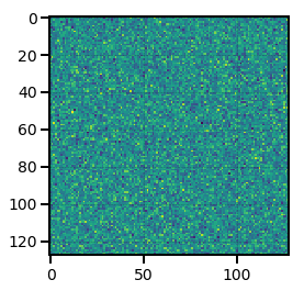
Gaussian Realizations
A Gaussian realization of a density field can be initialized directly
on a mesh using the LinearMesh class.
This class generates the Fourier modes of density field with a variance
set by an input power spectrum function. It allows the user to create
density fields with a known power spectrum, which is often a useful tool in
large-scale structure analysis.
Users can take advantage of the built-in linear power spectrum
class, LinearPower, or use their own
function to specify the desired power spectrum. The function should take
a single argument k, the wavenumber. Several transfer functions can be
used with the LinearPower class,
including from the CLASS CMB Boltzmann code, and the analytic fitting formulas from
Eisenstein and Hu 1998 with and without
Baryon Acoustic Oscillations.
In addition to the power spectrum function, users need to specify
a mesh size via the Nmesh parameter and a box size via the BoxSize
parameter. For example, to create
a density field on a mesh using the 2015 Planck cosmological parameters
and the Eisenstein-Hu linear power spectrum at redshift \(z=0\), use
[3]:
from nbodykit.lab import LinearMesh, cosmology
from matplotlib import pyplot as plt

cosmo = cosmology.Planck15
Plin = cosmology.LinearPower(cosmo, redshift=0, transfer='EisensteinHu')

# initialize the mesh
mesh = LinearMesh(Plin, Nmesh=128, BoxSize=1380, seed=42)

# preview the density field
plt.imshow(mesh.preview(axes=[0,1]))
[3]:
<matplotlib.image.AxesImage at 0x7f0b1af1b6d8>
From In-memory Data
From a RealField or ComplexField
If a pmesh.pm.RealField or pmesh.pm.ComplexField object
is already stored in memory, they can be converted easily into a mesh object
using the FieldMesh class. For example,
[4]:
from nbodykit.lab import FieldMesh
from pmesh.pm import RealField, ComplexField, ParticleMesh

# a 8^3 mesh
pm = ParticleMesh(Nmesh=[8,8,8])

# initialize a RealField
rfield = RealField(pm)

# set entire mesh to unity
rfield[...] = 1.0

# initialize from the RealField
real_mesh = FieldMesh(rfield)

# can also initialize from a ComplexField
cfield = rfield.r2c()
complex_mesh = FieldMesh(cfield)
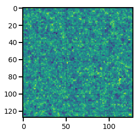
From a Numpy Array
Given a 3D numpy array stored in memory that represents data on a mesh, users
can initialize a mesh object using the
ArrayMesh class. The array for the full
mesh must be stored in memory on a single rank and not split in parallel across
multiple ranks. After initializing the ArrayMesh
object, the mesh data will be automatically spread out across the available ranks.
A common use case for this class is when a single rank handles the input/output
of the mesh data in the form of numpy arrays. Then, a single rank can read
in the array data from disk, and the mesh object can be initialized using
the ArrayMesh class.
For example,
[5]:
from nbodykit.lab import ArrayMesh
import numpy

# generate random data on a 128^3 mesh
data = numpy.random.random(size=(128,128,128))

# inititalize the mesh
mesh = ArrayMesh(data, BoxSize=1.0)

# preview the density mesh
plt.imshow(mesh.preview(axes=[0,1]))
[5]:
<matplotlib.image.AxesImage at 0x7f0b1aebf0b8>