The Power Spectrum of Data in a Simulation Box
In this notebook, we explore the functionality of the FFTPower algorithm, which can compute the 1D power spectrum \(P(k)\), 2D power spectrum \(P(k,\mu)\), and multipoles \(P_\ell(k)\). The algorithm is suitable for use on data sets in periodic simulation boxes, as the power spectrum is computed via a single FFT of the density mesh.
[1]:
%matplotlib inline
%config InlineBackend.figure_format = 'retina'
[2]:
from nbodykit.lab import *
from nbodykit import setup_logging, style

import matplotlib.pyplot as plt
plt.style.use(style.notebook)
[3]:
setup_logging()
Initalizing a Log-normal Mock
We start by generating a mock catalog of biased objects (\(b_1 = 2\) ) at a redshif \(z=0.55\). We use the Planck 2015 cosmology and the Eisenstein-Hu linear power spectrum fitting formula. We generate the catalog in a box of side length \(L = 1380 \ \mathrm{Mpc}/h\) with a constant number density \(\bar{n} = 3 \times 10^{-3} \ h^{3} \mathrm{Mpc}^{-3}\).
[4]:
redshift = 0.55
cosmo = cosmology.Planck15
Plin = cosmology.LinearPower(cosmo, redshift, transfer='EisensteinHu')
b1 = 2.0

cat = LogNormalCatalog(Plin=Plin, nbar=3e-4, BoxSize=1380., Nmesh=256, bias=b1, seed=42)
We update the Position column to add redshift-space distortions along the z axis of the box using the VelocityOffset column.
[5]:
# add RSD
line_of_sight = [0,0,1]
cat['RSDPosition'] = cat['Position'] + cat['VelocityOffset'] * line_of_sight
Computing the 1D Power, \(P(k)\)
In this section, we compute and plot the 1D power spectrum \(P(k)\) of the log-normal mock.
We must first convert our CatalogSource object to a MeshSource, by setting up the mesh and specifying which interpolation kernel we wish to use. Here, we use “TSC” interpolation, and specify via compensated=True that we wish to correct for the effects of the interpolation window in Fourier space.
[6]:
# convert to a MeshSource, using TSC interpolation on 256^3 mesh
mesh = cat.to_mesh(window='tsc', Nmesh=256, compensated=True, position='RSDPosition')
We compute the 1D power spectrum by specifying mode as “1d”. We also choose the desired linear k binning by specifying the bin spacing via dk and the minimum k value via kmin.
[7]:
# compute the power, specifying desired linear k-binning
r = FFTPower(mesh, mode='1d', dk=0.005, kmin=0.01)
[ 000010.90 ]   0: 10-30 20:44  CatalogMesh     INFO     painted 787121 out of 787121 objects to mesh
[ 000010.90 ]   0: 10-30 20:44  CatalogMesh     INFO     mean particles per cell is 0.0469161
[ 000010.91 ]   0: 10-30 20:44  CatalogMesh     INFO     sum is 787120
[ 000010.91 ]   0: 10-30 20:44  CatalogMesh     INFO     normalized the convention to 1 + delta
[ 000011.25 ]   0: 10-30 20:44  CatalogMesh     INFO     field: (LogNormalCatalog(seed=42, bias=2) as CatalogMesh) painting done
The result is computed when initializing the FFTPower class and the power spectrum results are stored as a BinnedStatistic object as the power attribute.
[8]:
# the result is stored at "power" attribute
Pk = r.power
print(Pk)
<BinnedStatistic: dims: (k: 115), variables: ('k', 'power', 'modes')>
The coords attribute of the BinnedStatistic object specifies the coordinate grid for the binned result, which in this case, is just the center values of the k bins.
By default, the power is computed up to the 1D Nyquist frequency, which is defined as \(k_\mathrm{Nyq} = \pi N_\mathrm{mesh} / L_\mathrm{box}\), which in this case is equal to \(k_\mathrm{Nyq} = \pi \cdot 256 / 1380 = 0.5825 \ h \ \mathrm{Mpc}^{-1}\).
[9]:
print(Pk.coords)
{'k': array([ 0.0125,  0.0175,  0.0225,  0.0275,  0.0325,  0.0375,  0.0425,
        0.0475,  0.0525,  0.0575,  0.0625,  0.0675,  0.0725,  0.0775,
        0.0825,  0.0875,  0.0925,  0.0975,  0.1025,  0.1075,  0.1125,
        0.1175,  0.1225,  0.1275,  0.1325,  0.1375,  0.1425,  0.1475,
        0.1525,  0.1575,  0.1625,  0.1675,  0.1725,  0.1775,  0.1825,
        0.1875,  0.1925,  0.1975,  0.2025,  0.2075,  0.2125,  0.2175,
        0.2225,  0.2275,  0.2325,  0.2375,  0.2425,  0.2475,  0.2525,
        0.2575,  0.2625,  0.2675,  0.2725,  0.2775,  0.2825,  0.2875,
        0.2925,  0.2975,  0.3025,  0.3075,  0.3125,  0.3175,  0.3225,
        0.3275,  0.3325,  0.3375,  0.3425,  0.3475,  0.3525,  0.3575,
        0.3625,  0.3675,  0.3725,  0.3775,  0.3825,  0.3875,  0.3925,
        0.3975,  0.4025,  0.4075,  0.4125,  0.4175,  0.4225,  0.4275,
        0.4325,  0.4375,  0.4425,  0.4475,  0.4525,  0.4575,  0.4625,
        0.4675,  0.4725,  0.4775,  0.4825,  0.4875,  0.4925,  0.4975,
        0.5025,  0.5075,  0.5125,  0.5175,  0.5225,  0.5275,  0.5325,
        0.5375,  0.5425,  0.5475,  0.5525,  0.5575,  0.5625,  0.5675,
        0.5725,  0.5775,  0.5825])}
The input parameters to the algorithm, as well as the meta-data computed during the calculation, are stored in the attrs dictionary attribute. A key attribute is the Poisson shot noise, stored as the “shotnoise” key.
[10]:
# print out the meta-data
for k in Pk.attrs:
    print("%s = %s" %(k, str(Pk.attrs[k])))
Nmesh = [256 256 256]
BoxSize = [ 1380.  1380.  1380.]
dk = 0.005
kmin = 0.01
Lx = 1380.0
Ly = 1380.0
Lz = 1380.0
volume = 2628072000.0
mode = 1d
los = [0, 0, 1]
Nmu = 1
poles = []
N1 = 787121
N2 = 787121
shotnoise = 3338.84116927
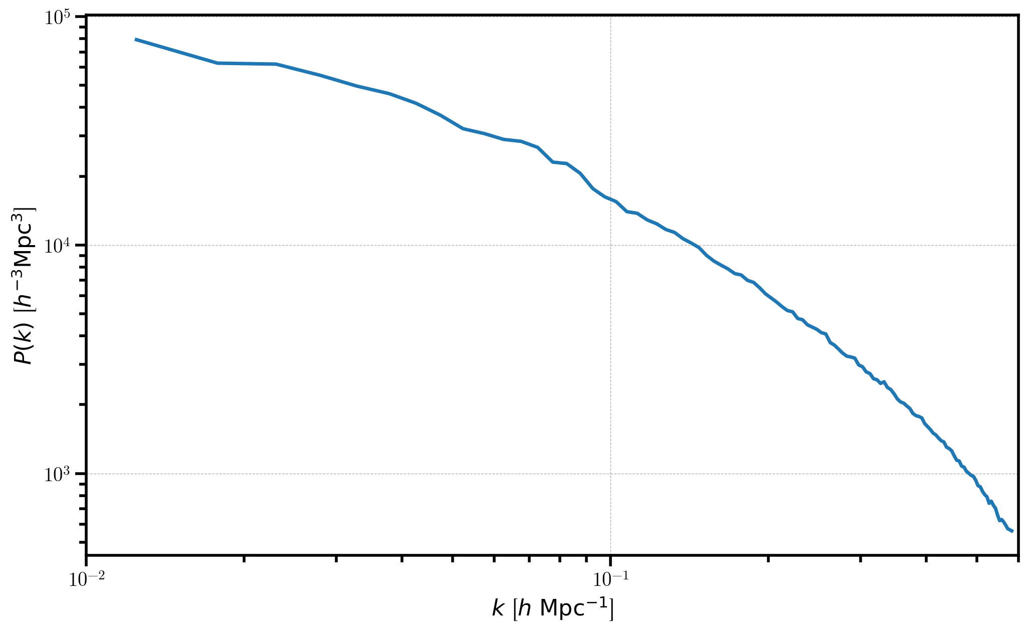
Now, we plot the 1D power, first subtracting out the shot noise. Note that the power is complex, so we only plot the real part.
[11]:
# print the shot noise subtracted P(k)
plt.loglog(Pk['k'], Pk['power'].real - Pk.attrs['shotnoise'])

# format the axes
plt.xlabel(r"$k$ [$h \ \mathrm{Mpc}^{-1}$]")
plt.ylabel(r"$P(k)$ [$h^{-3}\mathrm{Mpc}^3$]")
plt.xlim(0.01, 0.6)
[11]:
(0.01, 0.6)
Computing the 2D Power, \(P(k,\mu)\)
In this section, we compute and plot the 2D power spectrum \(P(k,\mu)\). For illustration, we compute results using a line-of-sight that is both parallel and perpendicular to the direction that we added redshift-space distortions.
Here, we compute \(P(k,\mu)\) where \(\mu\) is defined with respect to the z axis (los=[0,0,1]), using 5 \(\mu\) bins ranging from \(\mu=0\) to \(\mu=1\).
[12]:
# compute the 2D power
r = FFTPower(mesh, mode='2d', dk=0.005, kmin=0.01, Nmu=5, los=[0,0,1])
Pkmu = r.power
print(Pkmu)
[ 000014.28 ]   0: 10-30 20:44  CatalogMesh     INFO     painted 787121 out of 787121 objects to mesh
[ 000014.29 ]   0: 10-30 20:44  CatalogMesh     INFO     mean particles per cell is 0.0469161
[ 000014.29 ]   0: 10-30 20:44  CatalogMesh     INFO     sum is 787120
[ 000014.29 ]   0: 10-30 20:44  CatalogMesh     INFO     normalized the convention to 1 + delta
[ 000014.71 ]   0: 10-30 20:44  CatalogMesh     INFO     field: (LogNormalCatalog(seed=42, bias=2) as CatalogMesh) painting done
<BinnedStatistic: dims: (k: 115, mu: 5), variables: ('k', 'mu', 'power', 'modes')>
The coords attribute of the result now gives the centers of both the k and mu bins.
[13]:
print(Pkmu.coords)
{'k': array([ 0.0125,  0.0175,  0.0225,  0.0275,  0.0325,  0.0375,  0.0425,
        0.0475,  0.0525,  0.0575,  0.0625,  0.0675,  0.0725,  0.0775,
        0.0825,  0.0875,  0.0925,  0.0975,  0.1025,  0.1075,  0.1125,
        0.1175,  0.1225,  0.1275,  0.1325,  0.1375,  0.1425,  0.1475,
        0.1525,  0.1575,  0.1625,  0.1675,  0.1725,  0.1775,  0.1825,
        0.1875,  0.1925,  0.1975,  0.2025,  0.2075,  0.2125,  0.2175,
        0.2225,  0.2275,  0.2325,  0.2375,  0.2425,  0.2475,  0.2525,
        0.2575,  0.2625,  0.2675,  0.2725,  0.2775,  0.2825,  0.2875,
        0.2925,  0.2975,  0.3025,  0.3075,  0.3125,  0.3175,  0.3225,
        0.3275,  0.3325,  0.3375,  0.3425,  0.3475,  0.3525,  0.3575,
        0.3625,  0.3675,  0.3725,  0.3775,  0.3825,  0.3875,  0.3925,
        0.3975,  0.4025,  0.4075,  0.4125,  0.4175,  0.4225,  0.4275,
        0.4325,  0.4375,  0.4425,  0.4475,  0.4525,  0.4575,  0.4625,
        0.4675,  0.4725,  0.4775,  0.4825,  0.4875,  0.4925,  0.4975,
        0.5025,  0.5075,  0.5125,  0.5175,  0.5225,  0.5275,  0.5325,
        0.5375,  0.5425,  0.5475,  0.5525,  0.5575,  0.5625,  0.5675,
        0.5725,  0.5775,  0.5825]), 'mu': array([ 0.1,  0.3,  0.5,  0.7,  0.9])}
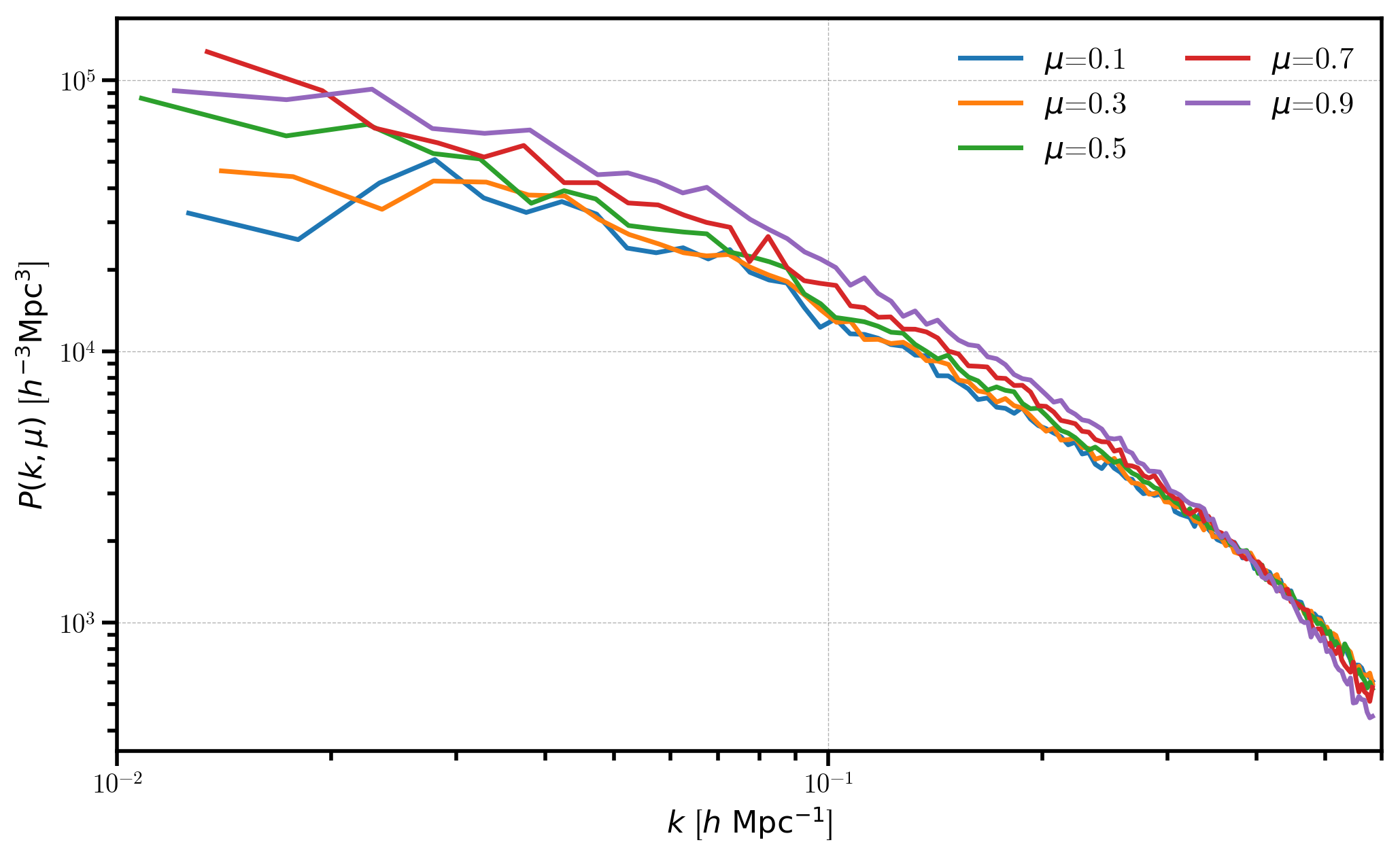
We plot each the power for each of the 5 \(\mu\) bins, and we see the effects of redshift-space distortions as a function of \(\mu\).
[14]:
# plot each mu bin
for i in range(Pkmu.shape[1]):
    Pk = Pkmu[:,i] # select the ith mu bin
    label = r'$\mu$=%.1f' % (Pkmu.coords['mu'][i])
    plt.loglog(Pk['k'], Pk['power'].real - Pk.attrs['shotnoise'], label=label)

# format the axes
plt.legend(loc=0, ncol=2)
plt.xlabel(r"$k$ [$h \ \mathrm{Mpc}^{-1}$]")
plt.ylabel(r"$P(k, \mu)$ [$h^{-3}\mathrm{Mpc}^3$]")
plt.xlim(0.01, 0.6)
[14]:
(0.01, 0.6)
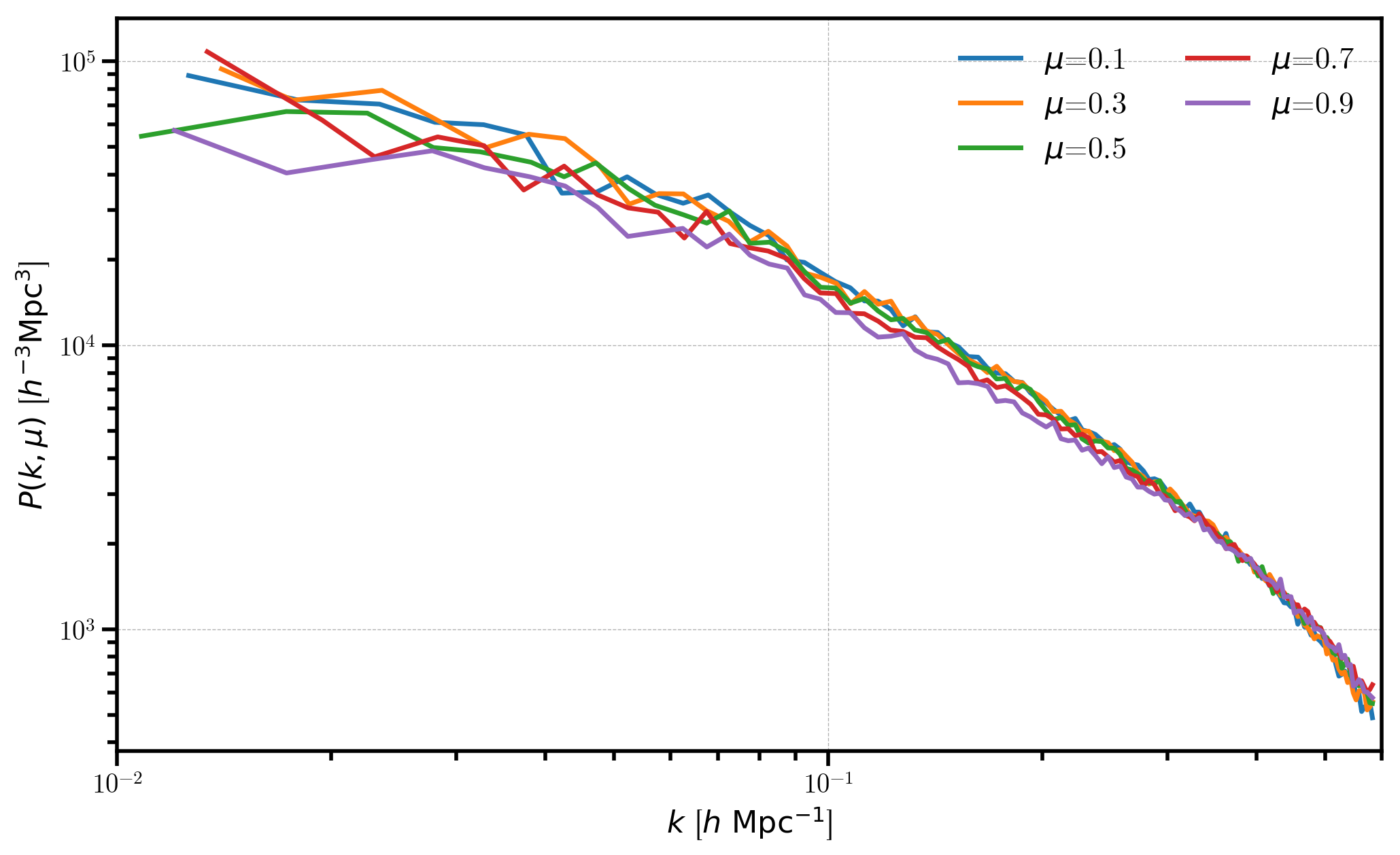
Now, we specify the line-of-sight as the x axis and again compute the 2D power.
[15]:
r = FFTPower(mesh, mode='2d', dk=0.005, kmin=0.01, Nmu=5, los=[1,0,0])
Pkmu = r.power
[ 000018.03 ]   0: 10-30 20:44  CatalogMesh     INFO     painted 787121 out of 787121 objects to mesh
[ 000018.03 ]   0: 10-30 20:44  CatalogMesh     INFO     mean particles per cell is 0.0469161
[ 000018.03 ]   0: 10-30 20:44  CatalogMesh     INFO     sum is 787120
[ 000018.03 ]   0: 10-30 20:44  CatalogMesh     INFO     normalized the convention to 1 + delta
[ 000018.45 ]   0: 10-30 20:44  CatalogMesh     INFO     field: (LogNormalCatalog(seed=42, bias=2) as CatalogMesh) painting done
Again we plot the 2D power for each of the \(\mu\) bins, but now that \(\mu\) is not defined along the same axis as the redshift-space distortions, we measure isotropic power as a function of \(\mu\).
[16]:
# plot each mu bin
for i in range(Pkmu.shape[1]):
    Pk = Pkmu[:,i] # select the ith mu bin
    label = r'$\mu$=%.1f' % (Pkmu.coords['mu'][i])
    plt.loglog(Pk['k'], Pk['power'].real - Pk.attrs['shotnoise'], label=label)

# format the axes
plt.legend(loc=0, ncol=2)
plt.xlabel(r"$k$ [$h \ \mathrm{Mpc}^{-1}$]")
plt.ylabel(r"$P(k, \mu)$ [$h^{-3}\mathrm{Mpc}^3$]")
plt.xlim(0.01, 0.6)
[16]:
(0.01, 0.6)
Computing the Multipoles, \(P_\ell(k)\)
In this section, we also measure the power spectrum multipoles, \(P_\ell\), which projects the 2D power on to a basis defined by Legendre weights. The desired multipole numbers \(\ell\) should be specified as the poles keyword.
[17]:
# compute the 2D power AND ell=0,2,4 multipoles
r = FFTPower(mesh, mode='2d', dk=0.005, kmin=0.01, Nmu=5, los=[0,0,1], poles=[0,2,4])
[ 000021.70 ]   0: 10-30 20:44  CatalogMesh     INFO     painted 787121 out of 787121 objects to mesh
[ 000021.70 ]   0: 10-30 20:44  CatalogMesh     INFO     mean particles per cell is 0.0469161
[ 000021.70 ]   0: 10-30 20:44  CatalogMesh     INFO     sum is 787120
[ 000021.70 ]   0: 10-30 20:44  CatalogMesh     INFO     normalized the convention to 1 + delta
[ 000022.04 ]   0: 10-30 20:44  CatalogMesh     INFO     field: (LogNormalCatalog(seed=42, bias=2) as CatalogMesh) painting done
Now, there is an additional attribute poles which stores the \(P_\ell(k)\) result.
[18]:
poles = r.poles
print(poles)
print("variables = ", poles.variables)
<BinnedStatistic: dims: (k: 115), variables: 5 total>
variables =  ['k', 'power_0', 'power_2', 'power_4', 'modes']
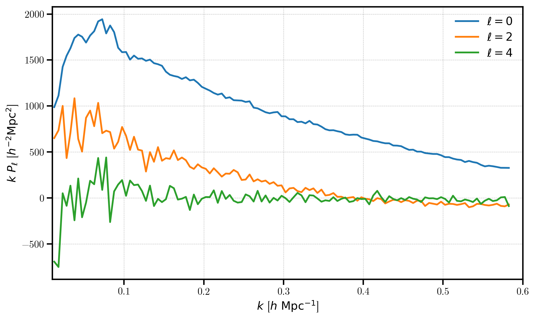
We plot each multipole, subtracting the shot noise only from the monopole \(P_0\). The multipoles are stored using the variable names “power_0”, “power_2”, etc for \(\ell=0,2,\) etc.
[19]:
for ell in [0, 2, 4]:
    label = r'$\ell=%d$' % (ell)
    P = poles['power_%d' %ell].real
    if ell == 0: P = P - poles.attrs['shotnoise']
    plt.plot(poles['k'], poles['k'] * P, label=label)

# format the axes
plt.legend(loc=0)
plt.xlabel(r"$k$ [$h \ \mathrm{Mpc}^{-1}$]")
plt.ylabel(r"$k \ P_\ell$ [$h^{-2} \mathrm{Mpc}^2$]")
plt.xlim(0.01, 0.6)
[19]:
(0.01, 0.6)