Common Mesh Operations
In this section, we detail some common operations for manipulating data
defined on a mesh via a MeshSource object.
Previewing the Mesh
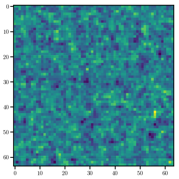
The MeshSource.preview() function allows users to preview a
low-resolution mesh by resampling the mesh and gathering the mesh to all
ranks. It can also optionally project the mesh across multiple axes, which
enables visualizations of the projected density field for quick data
inspection by the user.
For example, below we initialize a
LinearMesh object on a \(128^3\)
mesh and preview the mesh on a \(64^3\) mesh after projecting the field
along two axes:
In [2]:
from nbodykit.lab import LinearMesh, cosmology
from matplotlib import pyplot as plt

cosmo = cosmology.Planck15
Plin = cosmology.LinearPower(cosmo, redshift=0, transfer='EisensteinHu')

mesh = LinearMesh(Plin, Nmesh=128, BoxSize=1380, seed=42)

density = mesh.preview(Nmesh=64, axes=(0,1))
plt.imshow(density)
Out[2]:
<matplotlib.image.AxesImage at 0x1215b03c8>
Note
The previewed mesh result is broadcast to all ranks, so each rank allocates \(\mathrm{Nmesh}^3\) in memory.
Saving and Loading a Mesh
The MeshSource.save() function paints the mesh via a call to
MeshSource.paint() and saves the mesh using a bigfile format.
The output mesh saved to file can be in either configuration space or Fourier
space, by specifying mode as either real or complex.
Below, we save our LinearMesh to a
bigfile file:
In [3]:
# save the RealField
mesh.save('linear-mesh-real.bigfile', mode='real', dataset='Field')

# save the ComplexField
mesh.save('linear-mesh-complex.bigfile', mode='real', dataset='Field')
The saved mesh can be loaded from disk using the
BigFileMesh class:
In [4]:
from nbodykit.lab import BigFileMesh
import numpy

# load the mesh in the form of a RealField
real_mesh = BigFileMesh('linear-mesh-real.bigfile', 'Field')

# return the RealField via paint
rfield = real_mesh.paint(mode='real')

# load the mesh in the form of a ComplexField
complex_mesh = BigFileMesh('linear-mesh-complex.bigfile', 'Field')

# FFT to get the ComplexField as a RealField
rfield2 = complex_mesh.paint(mode='real')

# the two RealFields must be the same!
numpy.allclose(rfield.value, rfield2.value)
Out[4]:
True
Here, we load our meshes in configuration space and Fourier space and then
paint both with mode=real and verify that the results are the same.
Applying Functions to the Mesh
nbodykit supports performing transformations to the mesh data by applying
arbitrary functions in either configuration space or Fourier space. Users
can use the MeshSource.apply() function to apply these transformations.
The function applied to the mesh should take two arguments, x and v:
- The
xargument provides a list of length three holding the coordinate arrays that define the mesh. These arrays broadcast to the full shape of the mesh, i.e., they have shapes \((N_x,1,1)\), \((1,N_y,1)\), and \((1,1,N_z)\) if the mesh has shape \((N_x, N_y, N_z)\). - The
vargument is the array holding the value of the mesh field at the coordinate arrays inx
The units of the x coordinate arrays depend upon the values of the
kind and mode keywords passed to the apply() function.
The various cases are:
| mode | kind | range of the “x” argument |
real |
relative |
\([-L/2, L/2)\) |
real |
index |
\([0, N)\) |
complex |
wavenumber |
\([- \pi N/L, \pi N / L)\) |
complex |
circular |
\([-\pi, \pi)\) |
complex |
index |
\([0, N)\) |
Here, \(L\) is the size of the box and N is the number of cells per mesh side.
One common use of the MeshSource.apply() functionality is applying
compensation function to the mesh to correct for the interpolation window.
The table of built-in compensation functions in the
Compensation: Deconvolving the Window Kernel section provide examples of the syntax needed to apply
functions to the mesh.
In the example below, we apply a filter function in Fourier space that divides
the mesh by the squared norm of the wavenumber k on the mesh, and then
print out the first few mesh cells of the filtered mesh to verify the
function was applied properly.
In [5]:
def filter(k, v):
    kk = sum(ki ** 2 for ki in k) # k^2 on the mesh
    kk[kk == 0] = 1
    return v / kk # divide the mesh by k^2

# apply the filter and get a new mesh
filtered_mesh = mesh.apply(filter, mode='complex', kind='wavenumber')

# get the filtered RealField object
filtered_rfield = filtered_mesh.paint(mode='real')

print("head of filtered Realfield = ",  filtered_rfield[:10,0,0])
print("head of original RealField = ",  rfield[:10,0,0])
head of filtered Realfield =  [ 1094.85620117  1060.4699707   1058.02099609  1059.88293457  1067.56616211
  1104.82104492  1150.15161133  1193.57958984  1244.2277832   1295.75793457]
head of original RealField =  [ 0.14926976  0.8553862   1.73753595  2.27050304  1.69510484  1.92589998
  1.44721305  0.86124492  0.8651849   1.62193501]
Resampling a Mesh
Users can resample a mesh by specifying the Nmesh keyword to the
MeshSource.paint() function.
For example, below we resample a
LinearMesh object, changing the mesh
resolution from Nmesh=128 to Nmesh=32.
In [6]:
from nbodykit.lab import LinearMesh, cosmology

# linear mesh
Plin = cosmology.LinearPower(cosmology.Planck15, redshift=0.55, transfer='EisensteinHu')
source = LinearMesh(Plin, Nmesh=64, BoxSize=512, seed=42)

# paint, re-sampling to Nmesh=32
real = source.paint(mode='real', Nmesh=32)

print("original Nmesh = ", source.attrs['Nmesh'])
print("resampled Nmesh = ", real.Nmesh)
print("shape of resampled density field = ", real.cshape)
original Nmesh =  [64 64 64]
resampled Nmesh =  [32 32 32]
shape of resampled density field =  [32 32 32]