Mesh Interpolation Windows
In this notebook we explore the different window options for interpolating discrete objects on to a mesh. We compute the 1D power spectrum \(P(k)\) of a density field interpolated from a log-normal mock using different windows. The windows we test are:
- Cloud in Cell:
cic(default in nbodykit) - Triangular Shaped Cloud:
tsc - Lanczos Kernel
with \(a=2\) and \(a=3\):
lanczos2andlanczos3 - Symmetric Daubechies
wavelet with
sizes 6, 12, and 20:
sym6,sym12, andsym20
We also include timing tests when using each of these windows. The CIC window (default) is the fastest and can be considerably faster than the other kernels, especially the wavelet windows with large sizes.
When computing the power spectrum \(P(k)\), we de-convolve the
effects of the interpolation on the measured power
(compensated=True) for the CIC and TSC windows, but do not apply any
corrections for the other windows.
For more information on using the Daubechies wavelets for power spectrum measurements, see Cui et al. 2008.
In [1]:
%matplotlib inline
%config InlineBackend.figure_format = 'retina'
In [2]:
from nbodykit.lab import *
from nbodykit import style
from scipy.interpolate import InterpolatedUnivariateSpline as spline

import matplotlib.pyplot as plt
plt.style.use(style.notebook)
Initalizing a Log-normal Mock
We start by generating a mock catalog of biased objects (\(b_1 = 2\) ) at a redshif \(z=0.55\). We use the Planck 2015 cosmology and the Eisenstein-Hu linear power spectrum fitting formula. We generate the catalog in a box of side length \(L = 1380 \ \mathrm{Mpc}/h\) with a constant number density \(\bar{n} = 3 \times 10^{-3} \ h^{3} \mathrm{Mpc}^{-3}\).
In [3]:
redshift = 0.55
cosmo = cosmology.Planck15
Plin = cosmology.LinearPower(cosmo, redshift, transfer='EisensteinHu')

cat = LogNormalCatalog(Plin=Plin, nbar=3e-4, BoxSize=1380., Nmesh=256, bias=2.0, seed=42)
cat_noise = UniformCatalog(nbar=3e-4, BoxSize=1380., seed=42)
Generating the “Truth”
We generate the “truth” power spectrum by using a higher resolution mesh
with Nmesh=512, using the TSC window interpolation method. With a
higher resolution mesh, the Nyquist frequency is larger, decreasing the
effects of aliasing at a given \(k\) value.
In [4]:
r = FFTPower(cat.to_mesh(window='tsc', Nmesh=512, compensated=True),
            mode='1d') # hi-resolution mesh
truth = r.power
truth = spline(truth['k'], truth['power'].real - truth.attrs['shotnoise'])
The truth power of the Poisson shot noise is just \(\frac{1}{\bar{n}}\).
In [5]:
truth_noise = lambda k: 0.0 * k + 1 / 3e-4
Comparing Different Windows / LCDM-like
We compare the results when using different windows to measure a
LCDM-like \(P(k)\) as compared to the high-resolution “truth”
measured in the previous section. The goal is to identify which windows
perform better/worse at minimizing this differences. We compute results
using a lower-resultion mesh, Nmesh=256. The effects of aliasing are
clear: the measured power to differ from the “truth”. For CIC and TSC,
there is a residuel bias at small scale even after the resampling window
has been compensated. This is because the true power-spectrum is
LCDM-like, while the compensation window is derived for a shot-noise
like signal.
In [6]:
for window in ['cic', 'tsc', 'sym6', 'sym12', 'sym20', 'lanczos2', 'lanczos3']:

    print("computing power for window '%s'\n" %window + "-"*32)
    compensated = True if window in ['cic', 'tsc'] else False
    mesh = cat.to_mesh(Nmesh=256, window=window, compensated=compensated, interlaced=False)

    # compute the power
    %time r = FFTPower(mesh, mode='1d')
    Pk = r.power

    plt.plot(Pk['k'], (Pk['power'].real - Pk.attrs['shotnoise']) / truth(Pk['k']), label=window)

plt.legend(loc=0, ncol=2, fontsize=16)
plt.xlabel(r"$k$ [$h \ \mathrm{Mpc}^{-1}$]")
plt.ylabel(r"$P(k) / P(k)^\mathrm{truth}$")
plt.xlim(0.01, 0.6)
plt.ylim(0.9, 1.1)
computing power for window 'cic'
--------------------------------
CPU times: user 1.54 s, sys: 89.1 ms, total: 1.63 s
Wall time: 1.64 s
computing power for window 'tsc'
--------------------------------
CPU times: user 1.58 s, sys: 88.4 ms, total: 1.67 s
Wall time: 1.68 s
computing power for window 'sym6'
--------------------------------
CPU times: user 5.21 s, sys: 159 ms, total: 5.36 s
Wall time: 5.48 s
computing power for window 'sym12'
--------------------------------
CPU times: user 12.3 s, sys: 253 ms, total: 12.5 s
Wall time: 13 s
computing power for window 'sym20'
--------------------------------
CPU times: user 19.5 s, sys: 195 ms, total: 19.7 s
Wall time: 19.8 s
computing power for window 'lanczos2'
--------------------------------
CPU times: user 2.13 s, sys: 93.4 ms, total: 2.22 s
Wall time: 2.23 s
computing power for window 'lanczos3'
--------------------------------
CPU times: user 4.01 s, sys: 143 ms, total: 4.15 s
Wall time: 4.3 s
Out[6]:
(0.9, 1.1)
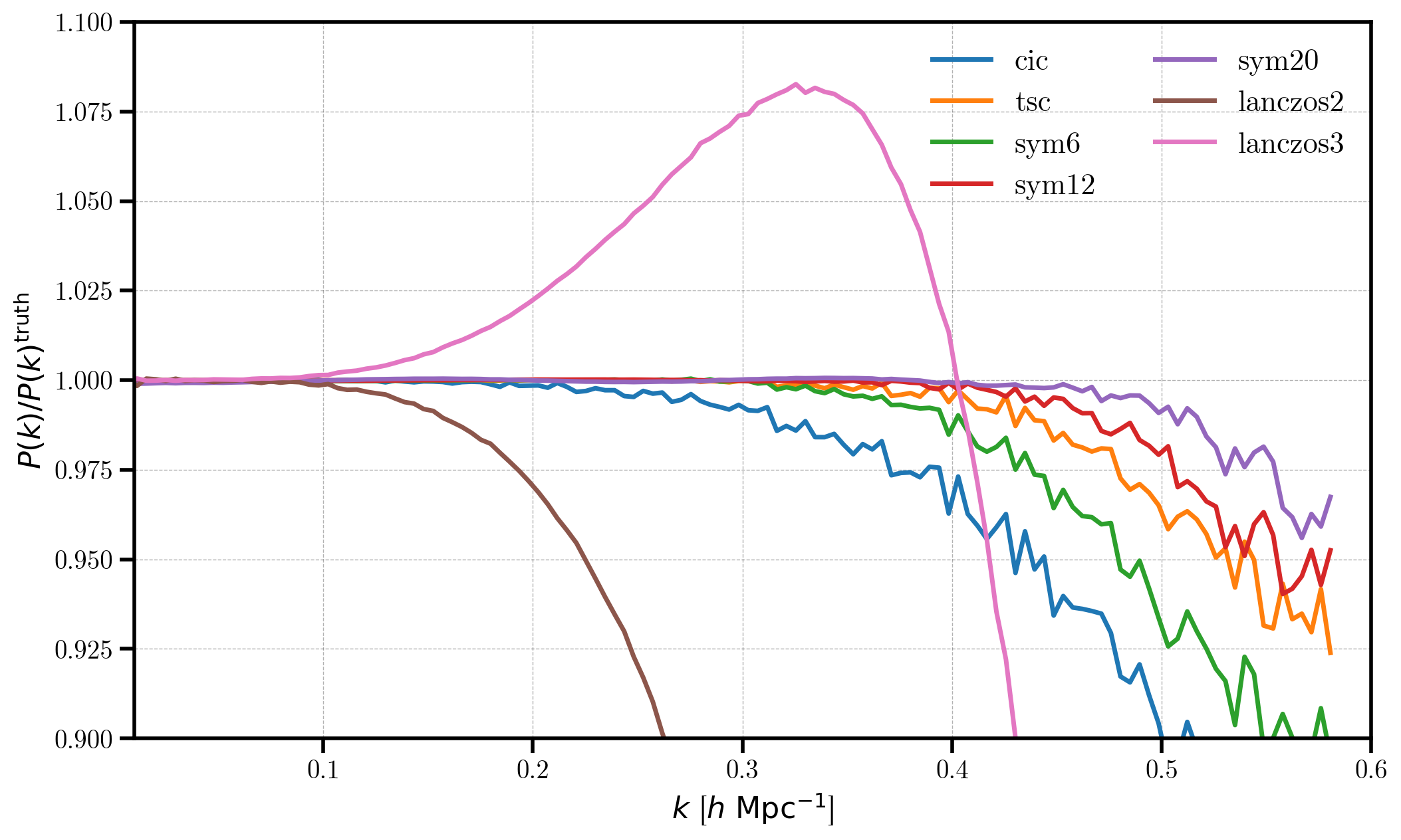
In this figure, we see that each window kernel has a specific
\(k_\mathrm{max}\) where we can reasonably trust the measured
results. The wavelet kernels sym12 and sym20 perform the best
but taking over an order magnitude longer to compute than the default
kernel (CIC). The Triangular Shaped Cloud window performs the next best,
followed by the sym6 kernel and the CIC kernel. The Lanczos kernels
do not perform well and should not be used by the user without
additional compensation corrections (currently not implemented by
default in nbodykit).
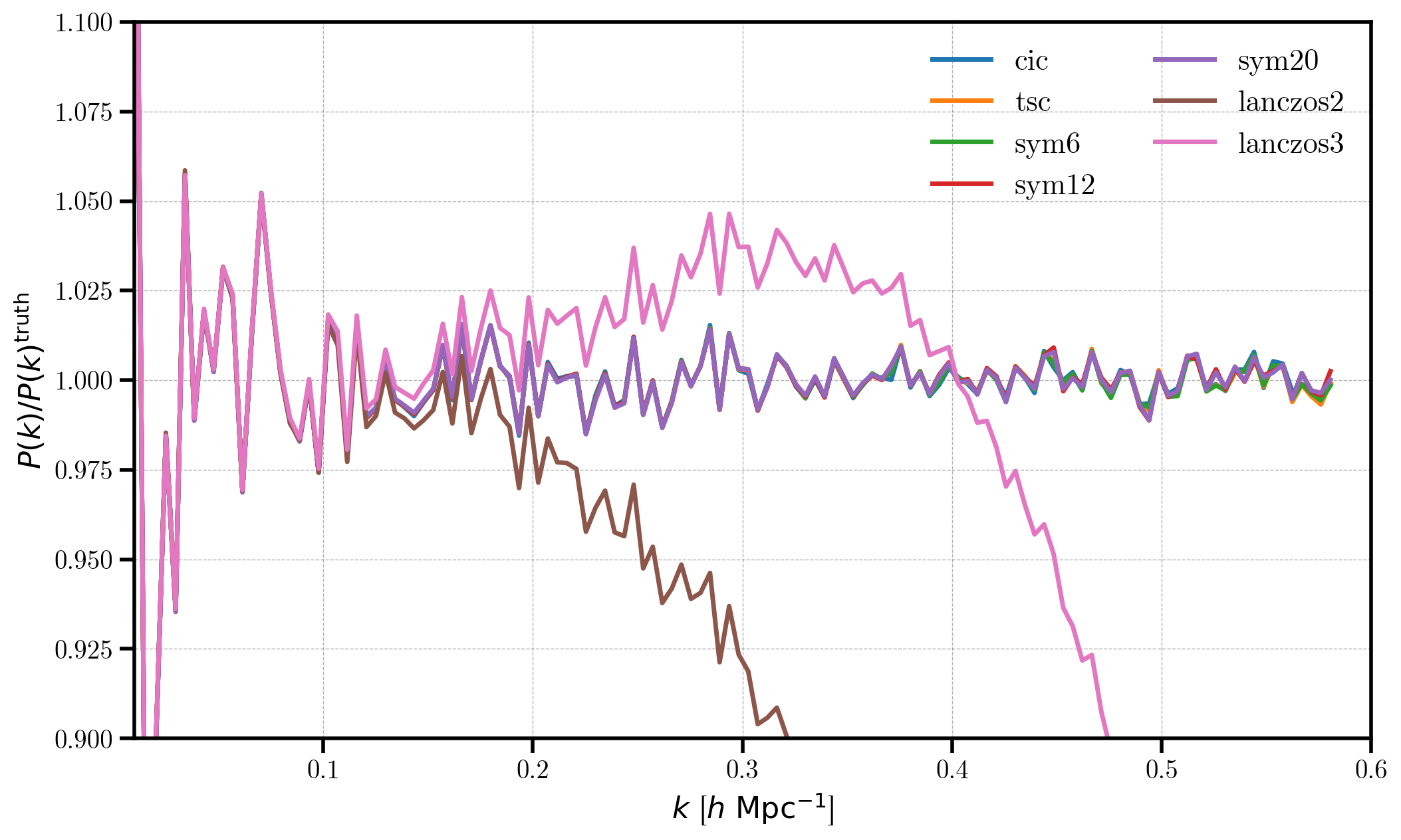
Comparing Different Windows / Shotnoise-like
We compare the results when using different windows to measure a
shotnois-like \(P(k)\) as compared to the high-resolution “truth”
measured in the previous section. We compute results using a
lower-resultion mesh, Nmesh=256. The effects of aliasing and
resampling is clear: compensation is effective at compensating the
‘missing’ power, recovering the flat shot-noise power. The wavelet
inspired resampling windows also recovers the shot-noise power
excellently. The lanczos based windows perform relatively badly due to a
lack of suitable compensation function.
In [7]:
for window in ['cic', 'tsc', 'sym6', 'sym12', 'sym20', 'lanczos2', 'lanczos3']:

    print("computing power for window '%s'\n" %window + "-"*32)
    compensated = True if window in ['cic', 'tsc'] else False
    mesh = cat_noise.to_mesh(Nmesh=256, window=window, compensated=compensated, interlaced=False)

    # compute the power
    %time r = FFTPower(mesh, mode='1d')
    Pk = r.power

    plt.plot(Pk['k'], (Pk['power'].real) / truth_noise(Pk['k']), label=window)

plt.legend(loc=0, ncol=2, fontsize=16)
plt.xlabel(r"$k$ [$h \ \mathrm{Mpc}^{-1}$]")
plt.ylabel(r"$P(k) / P(k)^\mathrm{truth}$")
plt.xlim(0.01, 0.6)
plt.ylim(0.9, 1.1)
computing power for window 'cic'
--------------------------------
CPU times: user 1.71 s, sys: 122 ms, total: 1.83 s
Wall time: 1.86 s
computing power for window 'tsc'
--------------------------------
CPU times: user 1.99 s, sys: 151 ms, total: 2.14 s
Wall time: 2.21 s
computing power for window 'sym6'
--------------------------------
CPU times: user 7.99 s, sys: 231 ms, total: 8.22 s
Wall time: 8.59 s
computing power for window 'sym12'
--------------------------------
CPU times: user 18.5 s, sys: 395 ms, total: 18.9 s
Wall time: 19.5 s
computing power for window 'sym20'
--------------------------------
CPU times: user 28.1 s, sys: 473 ms, total: 28.6 s
Wall time: 29.4 s
computing power for window 'lanczos2'
--------------------------------
CPU times: user 3.41 s, sys: 205 ms, total: 3.61 s
Wall time: 3.8 s
computing power for window 'lanczos3'
--------------------------------
CPU times: user 5.42 s, sys: 138 ms, total: 5.56 s
Wall time: 5.57 s
Out[7]:
(0.9, 1.1)
Recommendations
Given the increased speed costs of the wavelet windows, we recommend
users use either the CIC or TSC windows. For optimized solutions
providing the most precise results in the fastest amount of time, users
should test the effects of setting interlaced=True (see this
tutorial) while also trying various mesh sizes by
changing the Nmesh parameter. The most robust results are obtained
by running a series of convergence tests by computing results with a
high-resolution mesh, which reduces the contributions of aliasing at
fixed \(k\). This allows the user to robustly determine the best
configuration for their desired accuracy.