Cosmological Calculations
The nbodykit.cosmology module includes functionality for
representing cosmological parameter sets and computing various
theoretical quantities prevalent in large-scale structure that depend
on the background cosmological model. The module relies on the
CLASS CMB Boltzmann code as the underlying
engine for its cosmological calculations via the Python wrapper
provided by the classylss package. For consistency, the cosmology
syntax used in nbodykit largely follows that of the CLASS code. A useful
set of links for reference material on CLASS is available
here.
The Cosmology class
nbodykit provides the Cosmology
class for representing cosmological parameter sets. Given an input set of
parameters, this class uses the CLASS code to evaluate various quantities
relevant to large-scale structure. The class can compute background quantities,
such as distances, as a function of redshift, as well as linear and nonlinear
power spectra and transfer functions.
Note
For a full list of the attributes and functions available, please see the API docs.
The CLASS code supports multiple sets of input parameters, e.g., the user
can specify H0 or h. For simplicity, we use the following parameters
to initialize a Cosmology object:
h: the dimensionless Hubble parameterT0_cmb: the temperature of the CMB in KelvinsOmega0_b: the current baryon density parameter, \(\Omega_{b,0}\)Omega0_cdm: the current cold dark matter density parameter, \(\Omega_{cdm,0}\)N_ur: the number of ultra-relativistic (massless neutrino) speciesm_ncdm: the masses (in eV) for all massive neutrino speciesP_k_max: the maximum wavenumber to compute power spectrum results to, in units of \(h \mathrm{Mpc}^{-1}\)P_z_max: the maximum redshift to compute power spectrum results togauge: the General Relativity gauge, either “synchronous” or “newtonian”n_s: the tilt of the primordial power spectrumnonlinear: whether to compute nonlinear power spectrum results via HaloFit
Any valid CLASS parameters can be additionally specified as keywords to the
Cosmology constructor. If these additional parameters
conflict with the base set of parameters above, an exception will be raised.
For a guide to the valid input CLASS parameters, the “explanatory.ini”
parameter file in the CLASS GitHub is a good place to start.
Notes and Caveats
- The default configuration assumes a flat cosmology, \(\Omega_{k,0}=0\).
Pass
Omega0_kas a keyword to specify the desired non-flat curvature. - By default, the value for
N_uris inferred from the number of massive neutrinos using the following logic: if you have respectively 1,2,3 massive neutrinos and use the defaultT_ncdmvalue (0.71611 K), which is designed to give m/omega of 93.14 eV, and you wish to haveN_eff=3.046in the early universe, thenN_uris set to 2.0328, 1.0196, 0.00641, respectively. - For consistency of variable names, the present day values can be passed
with or without the “0” postfix, e.g.,
Omega0_cdmis translated toOmega_cdmas CLASS always uses the names without “0” as input parameters. - By default, a cosmological constant (
Omega0_lambda) is assumed, with its density value inferred by the curvature condition. - Non-cosmological constant dark energy can be used by specifying the
w0_fld,wa_fld, and/orOmega0_fldvalues. - To pass in CLASS parameters that are not valid Python argument names, use
the dictionary/keyword arguments trick, e.g.,
Cosmology(..., **{'temperature contributions': 'y'})
Builtin Cosmologies
We include several builtin cosmologies for users, accessible from the nbodykit.cosmology module:
| Name | Source | \(H_0\) | \(\Omega_{m,0}\) | Flat |
|---|---|---|---|---|
WMAP5 |
Komatsu et al. 2009 | 70.2 | 0.277 | Yes |
WMAP7 |
Komatsu et al. 2011 | 70.4 | 0.272 | Yes |
WMAP9 |
Hinshaw et al. 2013 | 69.3 | 0.287 | Yes |
Planck13 |
Planck Collab 2013, Paper XVI | 67.8 | 0.307 | Yes |
Planck15 |
Planck Collab 2015, Paper XIII | 67.7 | 0.307 | Yes |
Updating cosmological parameters
The Cosmology class is immutable. To update cosmological parameters,
we provide the following functions:
clone(): provides a newCosmologyobject with only the specified parameters changed; this function accepts any keyword parameters that can be passed to theCosmologyconstructormatch(): provides a newCosmologyobject that has matched a specific, derived parameter value. The derived parameters that can be matched include:sigma8: re-scale the scalar amplitudeA_sto matchsigma8Omega0_cb: match the total sum of cdm and baryons density, \(\Omega_{cdm,0}+\Omega_{b,0}\)Omega0_m: match the total density of matter-like components, \(\Omega_{cdm,0}+\Omega_{b,0}+\Omega_{ncdm,0}-\Omega_{pncdm,0}+\Omega_{dcdm,0}\)
For example, we can match a specific sigma8 value using:
In [2]:
from nbodykit.lab import cosmology

cosmo = cosmology.Cosmology()
print("original sigma8 = %.4f" % cosmo.sigma8)

new_cosmo = cosmo.match(sigma8=0.82)
print("new sigma8 = %.4f" % new_cosmo.sigma8)
original sigma8 = 0.8380
new sigma8 = 0.8200
And we can clone a Cosmology using
In [3]:
cosmo = cosmo.clone(h=0.7, nonlinear=True)
Converting to a dictionary
The keyword parameters passed to the constructor of a Cosmology object are not passed directly to the underlying CLASS engine, but must be edited first to be compatible with CLASS. Users can access the full set of parameters passed directly to CLASS by converting the Cosmology object to a dict. This can be accomplished simply using:
In [4]:
cosmo_dict = dict(cosmo)
print(cosmo_dict)
{'output': 'vTk dTk mPk', 'extra metric transfer functions': 'y', 'n_s': 0.9667, 'gauge': 'synchronous', 'N_ur': 2.0328, 'T_cmb': 2.7255, 'Omega_cdm': 0.26377065934278865, 'Omega_b': 0.0482754208891869, 'N_ncdm': 1, 'P_k_max_h/Mpc': 10.0, 'z_max_pk': 100.0, 'h': 0.7, 'm_ncdm': [0.06], 'non linear': 'halofit'}
Each of the parameters in this dictionary are valid CLASS parameters. For example, we see that the CLASS parameter “non linear” has been set to “halofit”, since we have set the nonlinear parameter to be True.
Note
To create a new Cosmology object from a dictionary, users should use
Cosmology.from_dict(dict(c)). Because of the differences in syntax between the Cosmology constructor
and CLASS, the following will not work: Cosmology(**dict(c)).
Interfacing with astropy
We provide some comptability for interfacing with the astropy.cosmology module. The following functions
of the Cosmology() class allow users to convert between the nbodykit and astropy cosmology
implementations:
to_astropy() |
Initialize and return a subclass of astropy.cosmology.FLRW from the Cosmology class. |
from_astropy(cosmo, **kwargs) |
Initialize and return a Cosmology object from a subclass of astropy.cosmology.FLRW. |
We also provide support for some of the syntax used by astropy for attributes in its cosmology classes by aliasing the astropy names to the appropriate nbodykit attributes. For example,
Om0 |
Returns Omega0_m. |
Odm0 |
Returns Omega0_cdm. |
Ode0 |
Returns the sum of Omega0_lambda and Omega0_fld. |
Ob0 |
Returns Omega0_b. |
Warning
The conversion between astropy and nbodykit cosmology objects is not one-to-one, as the classes are
implemented using different underlying engines. For example, the neutrino calculations performed in nbodykit
using CLASS differ from those in astropy. We have attempted to provide as much compatibility as possible,
but these differences will always remain when converting between the two implementations.
Theoretical Power Spectra
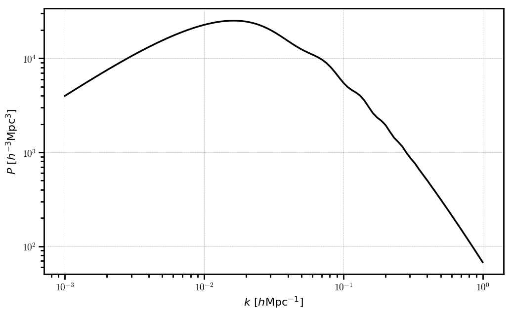
Linear power
The linear power spectrum can be computed for a given Cosmology and redshift using the LinearPower class. This object can compute the linear power spectrum using one of
several transfer functions:
- “CLASS”: calls CLASS to evaluate the total density transfer function at the specified redshift
- “EisensteinHu”: uses the analytic transfer function from Eisenstein & Hu, 1998
- “NoWiggleEisensteinHu”: uses the no-BAO analytic transfer function from Eisenstein & Hu, 1998
The LinearPower object is a callable function, taking wavenumber in units of \(h \mathrm{Mpc}^{-1}\) as input:
In [5]:
import matplotlib.pyplot as plt
import numpy as np

c = cosmology.Planck15
Plin = cosmology.LinearPower(c, redshift=0., transfer='CLASS')

k = np.logspace(-3, 0, 100)
plt.loglog(k, Plin(k), c='k')

plt.xlabel(r"$k$ $[h \mathrm{Mpc}^{-1}]$")
plt.ylabel(r"$P$ $[h^{-3} \mathrm{Mpc}^{3}]$")
plt.show()
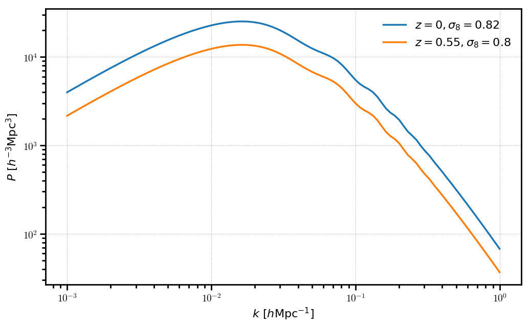
The redshift and power spectrum normalization can easily be updated by adjusting the redshift and sigma8 attributes of the LinearPower instance. For example,
In [6]:
# original power
plt.loglog(k, Plin(k), label=r"$z=0, \sigma_8=%.2f$" % Plin.sigma8)

# update the redshift and sigma8
Plin.redshift = 0.55
Plin.sigma8 = 0.80
plt.loglog(k, Plin(k), label=r"$z=0.55, \sigma_8=0.8$")

# format the axes
plt.legend()
plt.xlabel(r"$k$ $[h \mathrm{Mpc}^{-1}]$")
plt.ylabel(r"$P$ $[h^{-3} \mathrm{Mpc}^{3}]$")
plt.show()
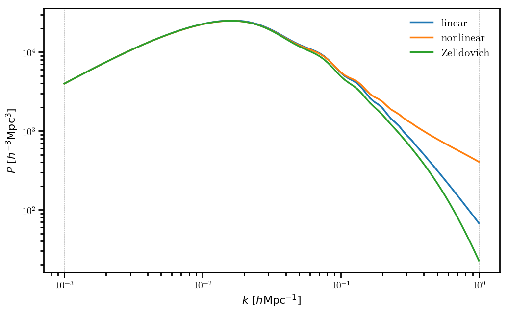
Nonlinear and Zel’dovich power
We also provide the HalofitPower and ZeldovichPower classes to compute the nonlinear and Zel’dovich power spectra, respectively. The nonlinear power uses the HaloFit prescription that is available in CLASS. These objects behavior very similarly to the LinearPower class.
For example,
In [7]:
# initialize the power objects
Plin = cosmology.LinearPower(c, redshift=0, transfer='CLASS')
Pnl = cosmology.HalofitPower(c, redshift=0)
Pzel = cosmology.ZeldovichPower(c, redshift=0)

# plot each kind
plt.loglog(k, Plin(k), label='linear')
plt.loglog(k, Pnl(k), label='nonlinear')
plt.loglog(k, Pzel(k), label="Zel'dovich")

# format the axes
plt.legend()
plt.xlabel(r"$k$ $[h \mathrm{Mpc}^{-1}]$")
plt.ylabel(r"$P$ $[h^{-3} \mathrm{Mpc}^{3}]$")
plt.show()
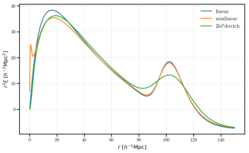
Correlation functions
nbodykit also includes functionality for computing theoretical correlation functions by computing the Fourier transform of a power spectrum. We use the mcfit package, which provides a Python version of the FFTLog algorithm. The main class to compute correlation functions is CorrelationFunction. This class
takes a power spectrum instance (one of LinearPower, HalofitPower,
or ZeldovichPower) as input. Below, we show the correlation function for each of these classes:
In [8]:
# initialize the correlation objects
cf_lin = cosmology.CorrelationFunction(Plin)
cf_nl = cosmology.CorrelationFunction(Pnl)
cf_zel = cosmology.CorrelationFunction(Pzel)

# plot each kind
r = np.logspace(-1, np.log10(150), 1000)
plt.plot(r, r**2 * cf_lin(r), label='linear')
plt.plot(r, r**2 * cf_nl(r), label='nonlinear')
plt.plot(r, r**2 * cf_zel(r), label="Zel'dovich")

# format the axes
plt.legend()
plt.xlabel(r"$r$ $[h^{-1} \mathrm{Mpc}]$")
plt.ylabel(r"$r^2 \xi \ [h^{-2} \mathrm{Mpc}^2]$")
plt.show()
We also include utility functions for performing the $P(k) leftrightarrow xi(r)$ transformation:
xi_to_pk(r, xi[, extrap]) |
Return a callable function returning the power spectrum, as computed from the Fourier transform of the input \(r\) and \(\xi(r)\) arrays. |
pk_to_xi(k, Pk[, extrap]) |
Return a callable function returning the correlation function, as computed from the Fourier transform of the input \(k\) and \(P(k)\) arrays. |
These functions take discretely evaluated \((r, \xi(r))\) or \((k, P(k))\) arrays and return a function that evaluates the appropriate transformed quantity.