Halo Occupation Distribution (HOD) Mocks
In this notebook, we will generate a mock halo catalog by running a FOF
finder on a LogNormalCatalog. We will then populate those halos with
galaxies via the HOD technique and compare the galaxy and halo power
spectra in both real and redshift space.
Note
When viewing results in this notebook, keep in mind that the FOF catalog
generated from the LogNormalCatalog object is only semi-realistic.
We choose to use the LogNormalCatalog rather than a more realistic
data set due to the ease with which we can load the mock data.
In [1]:
%matplotlib inline
%config InlineBackend.figure_format = 'retina'
In [2]:
from nbodykit.lab import *
from nbodykit import setup_logging, style

import matplotlib.pyplot as plt
plt.style.use(style.notebook)
In [3]:
setup_logging() # turn on logging to screen
Generating Halos via the FOF Algorithm
We’ll start by generating a mock galaxy catalog at \(z=0.55\) from a log-normal density field.
In [4]:
redshift = 0.55
cosmo = cosmology.Planck15
Plin = cosmology.EHPower(cosmo, redshift)
b1 = 2.0

input_cat = LogNormalCatalog(Plin=Plin, nbar=3e-3, BoxSize=1380., Nmesh=256, bias=b1, seed=42)
[ 000012.45 ] 0: 08-08 18:09 CatalogSource INFO total number of particles in LogNormalCatalog(seed=42, bias=2) = 7883861
And then, we run a friends-of-friends (FOF) algorithm on the mock galaxies to identify halos, using a linking length of 0.2 times the mean separation between objects. Here, we only keep halos with at least 5 particle members.
In [5]:
fof = FOF(input_cat, linking_length=0.2, nmin=5)
Now, we set the particle mass as \(10^{12} \ M_\odot/h\) and create
a HaloCatalog using the Planck 2015 parameters at a redshift of
\(z = 0.55\). Here, ‘vir’ specifies that we wish to create the
Mass column as the virial mass. This mass definition is necessary
for computing the analytic concentration, needed when generating the HOD
galaxies.
In [6]:
halos = fof.to_halos(cosmo=cosmo, redshift=redshift, particle_mass=1e12, mdef='vir')
[ 000038.43 ]   0: 08-08 18:10  CatalogSource   INFO     total number of particles in ArrayCatalog(size=24602) = 24602
[ 000038.43 ]   0: 08-08 18:10  CatalogSource   INFO     total number of particles in HaloCatalog(size=24602) = 24602
Finally, we convert the HaloCatalog object to a format recognized by
the halotools package and initialze our HOD catalog, using the
default HOD parameters.
In [7]:
halotools_halos = halos.to_halotools()
hod = HODCatalog(halotools_halos)
[ 000039.73 ]   0: 08-08 18:10  HOD             INFO     satellite fraction: 0.04
[ 000039.73 ]   0: 08-08 18:10  HOD             INFO     mean log10 halo mass: 13.10
[ 000039.73 ]   0: 08-08 18:10  HOD             INFO     std log10 halo mass: 0.30
[ 000039.73 ]   0: 08-08 18:10  HOD             INFO     total number of particles in HODCatalog(logMmin=13.03, sigma_logM=0.38, alpha=0.76, logM0=13.27, logM1=14.08) = 9505
Using the gal_type column, we can create subsets of the HOD catalog
that contain only centrals and only satellites.
In [8]:
cen_idx = hod['gal_type'] == 0
sat_idx = hod['gal_type'] == 1

cens = hod[cen_idx]
sats = hod[sat_idx]
[ 000039.76 ]   0: 08-08 18:10  CatalogSource   INFO     total number of particles in CatalogCopy(size=9129) = 9129
[ 000039.78 ]   0: 08-08 18:10  CatalogSource   INFO     total number of particles in CatalogCopy(size=376) = 376
Real-space Power Spectra
In this section, we compute the real-space power spectrum of the FOF halos and the HOD galaxies and compare.
In [9]:
# compute P(k) for the FOF halos
halo_power = FFTPower(halos, mode='1d', Nmesh=512)
[ 000039.80 ]   0: 08-08 18:10  CatalogMesh     INFO     total number of particles in (HaloCatalog(size=24602) as CatalogMesh) = 24602
[ 000040.44 ]   0: 08-08 18:10  CatalogMesh     INFO     painted 24602 out of 24602 objects to mesh
[ 000040.44 ]   0: 08-08 18:10  CatalogMesh     INFO     mean particles per cell is 0.000183299
[ 000040.44 ]   0: 08-08 18:10  CatalogMesh     INFO     sum is 24602
[ 000040.44 ]   0: 08-08 18:10  CatalogMesh     INFO     normalized the convention to 1 + delta
[ 000044.98 ]   0: 08-08 18:10  CatalogMesh     INFO     field: (HaloCatalog(size=24602) as CatalogMesh) painting done
And we can compute P(k) for all galaxies, centrals only, satellites only, and the cross power between centrals and satellites.
In [10]:
gal_power = FFTPower(hod, mode='1d', Nmesh=256)
cen_power = FFTPower(cens, mode='1d', Nmesh=256)
sat_power = FFTPower(sats, mode='1d', Nmesh=256)
cen_sat_power = FFTPower(cens, second=sats, mode='1d', Nmesh=256)
[ 000052.21 ]   0: 08-08 18:10  CatalogMesh     INFO     total number of particles in (HODCatalog(logMmin=13.03, sigma_logM=0.38, alpha=0.76, logM0=13.27, logM1=14.08) as CatalogMesh) = 9505
[ 000052.31 ]   0: 08-08 18:10  CatalogMesh     INFO     painted 9505 out of 9505 objects to mesh
[ 000052.31 ]   0: 08-08 18:10  CatalogMesh     INFO     mean particles per cell is 0.000566542
[ 000052.31 ]   0: 08-08 18:10  CatalogMesh     INFO     sum is 9505
[ 000052.31 ]   0: 08-08 18:10  CatalogMesh     INFO     normalized the convention to 1 + delta
[ 000052.87 ]   0: 08-08 18:10  CatalogMesh     INFO     field: (HODCatalog(logMmin=13.03, sigma_logM=0.38, alpha=0.76, logM0=13.27, logM1=14.08) as CatalogMesh) painting done
[ 000053.74 ]   0: 08-08 18:10  CatalogMesh     INFO     total number of particles in (CatalogCopy(size=9129) as CatalogMesh) = 9129
[ 000053.82 ]   0: 08-08 18:10  CatalogMesh     INFO     painted 9129 out of 9129 objects to mesh
[ 000053.83 ]   0: 08-08 18:10  CatalogMesh     INFO     mean particles per cell is 0.000544131
[ 000053.83 ]   0: 08-08 18:10  CatalogMesh     INFO     sum is 9129
[ 000053.83 ]   0: 08-08 18:10  CatalogMesh     INFO     normalized the convention to 1 + delta
[ 000054.33 ]   0: 08-08 18:10  CatalogMesh     INFO     field: (CatalogCopy(size=9129) as CatalogMesh) painting done
[ 000055.19 ]   0: 08-08 18:10  CatalogMesh     INFO     total number of particles in (CatalogCopy(size=376) as CatalogMesh) = 376
[ 000055.28 ]   0: 08-08 18:10  CatalogMesh     INFO     painted 376 out of 376 objects to mesh
[ 000055.28 ]   0: 08-08 18:10  CatalogMesh     INFO     mean particles per cell is 2.24113e-05
[ 000055.28 ]   0: 08-08 18:10  CatalogMesh     INFO     sum is 376
[ 000055.28 ]   0: 08-08 18:10  CatalogMesh     INFO     normalized the convention to 1 + delta
[ 000055.77 ]   0: 08-08 18:10  CatalogMesh     INFO     field: (CatalogCopy(size=376) as CatalogMesh) painting done
[ 000056.59 ]   0: 08-08 18:10  CatalogMesh     INFO     total number of particles in (CatalogCopy(size=9129) as CatalogMesh) = 9129
[ 000056.59 ]   0: 08-08 18:10  CatalogMesh     INFO     total number of particles in (CatalogCopy(size=376) as CatalogMesh) = 376
[ 000056.67 ]   0: 08-08 18:10  CatalogMesh     INFO     painted 9129 out of 9129 objects to mesh
[ 000056.67 ]   0: 08-08 18:10  CatalogMesh     INFO     mean particles per cell is 0.000544131
[ 000056.67 ]   0: 08-08 18:10  CatalogMesh     INFO     sum is 9129
[ 000056.67 ]   0: 08-08 18:10  CatalogMesh     INFO     normalized the convention to 1 + delta
[ 000057.17 ]   0: 08-08 18:10  CatalogMesh     INFO     field: (CatalogCopy(size=9129) as CatalogMesh) painting done
[ 000057.25 ]   0: 08-08 18:10  CatalogMesh     INFO     painted 376 out of 376 objects to mesh
[ 000057.25 ]   0: 08-08 18:10  CatalogMesh     INFO     mean particles per cell is 2.24113e-05
[ 000057.25 ]   0: 08-08 18:10  CatalogMesh     INFO     sum is 376
[ 000057.25 ]   0: 08-08 18:10  CatalogMesh     INFO     normalized the convention to 1 + delta
[ 000057.74 ]   0: 08-08 18:10  CatalogMesh     INFO     field: (CatalogCopy(size=376) as CatalogMesh) painting done
In [11]:
# plot galaxy auto power, centrals auto power, and sats auto power
labels = [r"$P^{gg}$", r"$P^{cc}$", r"$P^{ss}$"]
for i, r in enumerate([gal_power, cen_power, sat_power]):
    Pk = r.power
    plt.loglog(Pk['k'], Pk['power'].real-Pk.attrs['shotnoise'], label=labels[i])

# central-satellite power
Pk = cen_sat_power.power
plt.loglog(Pk['k'], Pk['power'].real, label=r"$P^{cs}$")

# the halo power
Phalo = halo_power.power
plt.loglog(Phalo['k'], Phalo['power'].real-Phalo.attrs['shotnoise'], c='k', label=r"$P^\mathrm{halo}$")

# add a legend and axis labels
plt.legend(loc=0, ncol=2)
plt.xlabel(r"$k$ [$h \ \mathrm{Mpc}^{-1}$]")
plt.ylabel(r"$P(k)$ [$h^{-3}\mathrm{Mpc}^3$]")
plt.xlim(0.01, 0.6)
plt.ylim(1e4, 5e6)
Out[11]:
(10000.0, 5000000.0)
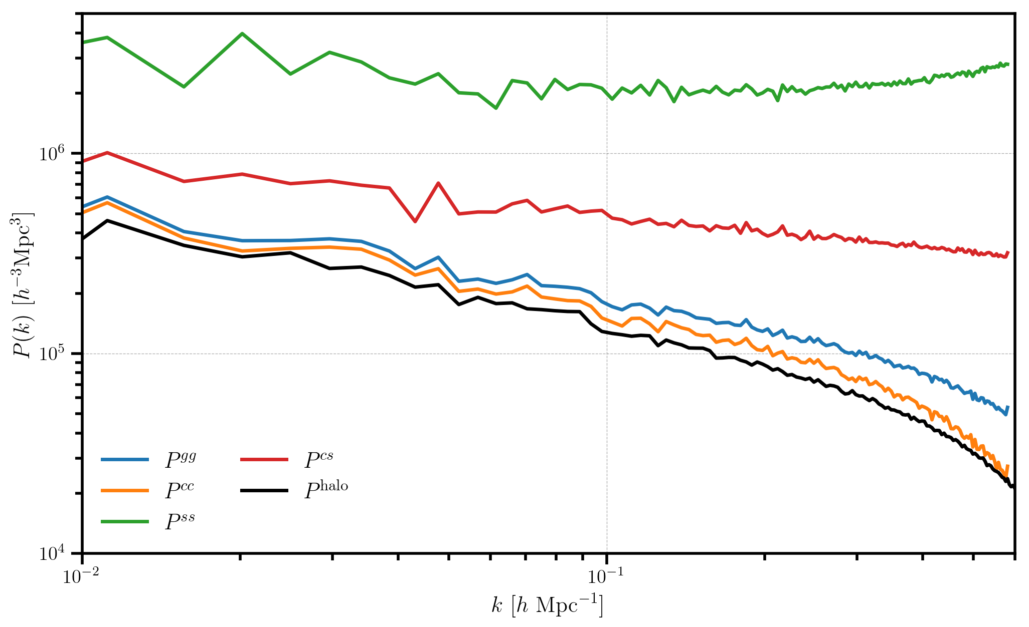
Here, we see the high bias of the satellite power spectrum (green). Because the satellite fraction is relatively low (\(f_\mathrm{sat} \simeq 0.04\)), the amplitude of the total galaxy power \(P^{gg}\) is only slightly larger than the centrals auto power \(P^{cc}\) – the centrals dominate the clustering signal.
Redshift-space Power Spectra
First, we convert HOD galaxy positions from real to redshift space.
In [12]:
LOS = [0, 0, 1]
hod['RSDPosition'] = hod['Position'] + hod['VelocityOffset'] * LOS
And then compute \(P(k,\mu)\) for the full HOD galaxy catalog in five \(\mu\) bins.
In [13]:
mesh = hod.to_mesh(position='RSDPosition', Nmesh=256, compensated=True)
rsd_gal_power = FFTPower(mesh, mode='2d', Nmu=5)
[ 000060.41 ]   0: 08-08 18:10  CatalogMesh     INFO     total number of particles in (HODCatalog(logMmin=13.03, sigma_logM=0.38, alpha=0.76, logM0=13.27, logM1=14.08) as CatalogMesh) = 9505
[ 000060.46 ]   0: 08-08 18:10  CatalogMesh     INFO     painted 9505 out of 9505 objects to mesh
[ 000060.46 ]   0: 08-08 18:10  CatalogMesh     INFO     mean particles per cell is 0.000566542
[ 000060.46 ]   0: 08-08 18:10  CatalogMesh     INFO     sum is 9505
[ 000060.46 ]   0: 08-08 18:10  CatalogMesh     INFO     normalized the convention to 1 + delta
[ 000060.78 ]   0: 08-08 18:10  CatalogMesh     INFO     field: (HODCatalog(logMmin=13.03, sigma_logM=0.38, alpha=0.76, logM0=13.27, logM1=14.08) as CatalogMesh) painting done
Finally, plot the galaxy \(P(k,\mu)\) and compare to the measured halo power in real space.
In [14]:
pkmu = rsd_gal_power.power

# plot each mu bin
for i in range(pkmu.shape[1]):
    Pk = pkmu[:,i]
    label = r'$P^{gg}(\mu$=%.1f)' %pkmu.coords['mu'][i]
    plt.loglog(Pk['k'], Pk['power'].real - Pk.attrs['shotnoise'], label=label)

# the halo power
Phalo = halo_power.power
plt.loglog(Phalo['k'], Phalo['power'].real-Phalo.attrs['shotnoise'], c='k', label=r"$P^\mathrm{halo}$")

# add a legend and axis labels
plt.legend(loc=0, ncol=2)
plt.xlabel(r"$k$ [$h \ \mathrm{Mpc}^{-1}$]")
plt.ylabel(r"$P(k, \mu)$ [$h^{-3}\mathrm{Mpc}^3$]")
plt.xlim(0.01, 0.6)
plt.ylim(1e4, 2e6)
Out[14]:
(10000.0, 2000000.0)
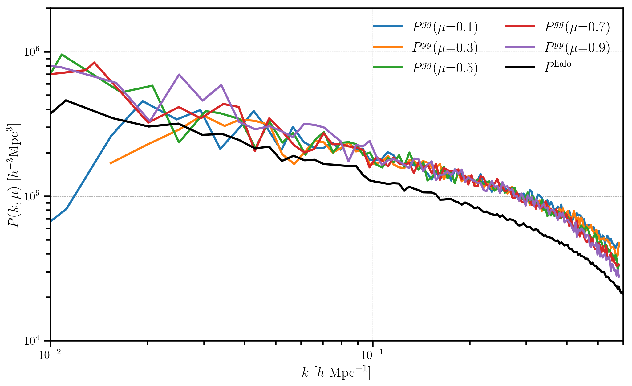
In this figure, we see the effects of RSD on the HOD catalog, with the power spectrum damped at higher \(\mu\) on small scales (larger \(k\)).