The Multipoles of the BOSS DR12 Dataset
In this notebook, we use the ConvolvedFFTPower algorithm to compute
the monopole, quadrupole, and hexadecapole of the BOSS DR12 LOWZ South
Galactic Cap (SGC) galaxy sample. This data set is described in detail
in Reid et al. 2016, and the
cosmological results for the BOSS DR12 data are presented in Alam et
al. 2017.
Here, we measure the power spectrum multipoles for the SGC LOWZ sample due to its relatively small size, such that this notebook can be executed in reasonable time on a laptop. The analysis presented in this notebook can easily be applied to the BOSS DR12 CMASS sample and samples in both the North and South Galactic Cap regions.
The BOSS dataset includes both the “data” and the “randoms” catalogs, each of which includes FKP weights, completeness weights, and \(n(z)\) values. This notebook illustrates how to incorporate these analysis steps into the power spectrum analysis using nbodykit.
In [1]:
%matplotlib inline
%config InlineBackend.figure_format = 'retina'
In [2]:
from nbodykit.lab import *
from nbodykit import setup_logging, style

import os
import matplotlib.pyplot as plt
plt.style.use(style.notebook)
In [3]:
setup_logging() # turn on logging to screen
Getting the Data
The BOSS DR12 galaxy data sets are available for download on the SDSS DR12 homepage. The “data” and “randoms” catalogs for the North Galactic CMASS sample are available from the following links:
- data: https://data.sdss.org/sas/dr12/boss/lss/galaxy_DR12v5_LOWZ_South.fits.gz (32.3 MB)
- randoms: https://data.sdss.org/sas/dr12/boss/lss/random0_DR12v5_LOWZ_South.fits.gz (713.3 MB)
After downloading the files, be sure to decompress them into the original FITS format.
Loading the Data from Disk
The “data” and “randoms” catalogs are stored on disk as FITS objects,
and we can use the FITSCatalog object to read the data from disk.
Note that the IO operations are performed on-demand, so no data is read from disk until an algorithm requires it to be read. For more details, see the On-Demand IO section of the documentation.
Note
To specify the directory where the BOSS catalogs were downloaded, change
the path_to_catalogs variable below.
In [4]:
# change this to the directory where the data was downloaded (default is current working directory)
path_to_catalogs = ""


# initialize the FITS catalog objects for data and randoms
data = FITSCatalog(os.path.join(path_to_catalogs, 'galaxy_DR12v5_LOWZ_South.fits'))
randoms = FITSCatalog(os.path.join(path_to_catalogs, 'random0_DR12v5_LOWZ_South.fits'))
[ 000000.01 ]   0: 08-08 18:07  CatalogSource   INFO     Extra arguments to FileType: ('galaxy_DR12v5_LOWZ_South.fits',)
[ 000000.01 ]   0: 08-08 18:07  CatalogSource   INFO     total number of particles in FITSCatalog(size=145264, file='galaxy_DR12v5_LOWZ_South.fits') = 145264
[ 000000.01 ]   0: 08-08 18:07  CatalogSource   INFO     Extra arguments to FileType: ('random0_DR12v5_LOWZ_South.fits',)
[ 000000.02 ]   0: 08-08 18:07  CatalogSource   INFO     total number of particles in FITSCatalog(size=7084128, file='random0_DR12v5_LOWZ_South.fits') = 7084128
We can analyze the available columns in the catalogs via the columns
attribute:
In [5]:
print('data columns = ', data.columns)
data columns = ['AIRMASS', 'CAMCOL', 'COMP', 'DEC', 'DEVFLUX', 'EB_MINUS_V', 'EXPFLUX', 'EXTINCTION', 'FIBER2FLUX', 'FIBERID', 'FIELD', 'FINALN', 'FRACPSF', 'ICHUNK', 'ICOLLIDED', 'ID', 'IMAGE_DEPTH', 'IMATCH', 'INGROUP', 'IPOLY', 'ISECT', 'MJD', 'MODELFLUX', 'MULTGROUP', 'NZ', 'PLATE', 'PSFFLUX', 'PSF_FWHM', 'RA', 'RERUN', 'RUN', 'R_DEV', 'SKYFLUX', 'SPECTILE', 'Selection', 'TILE', 'Value', 'WEIGHT_CP', 'WEIGHT_FKP', 'WEIGHT_NOZ', 'WEIGHT_SEEING', 'WEIGHT_STAR', 'WEIGHT_SYSTOT', 'Weight', 'Z']
In [6]:
print('randoms columns = ', randoms.columns)
randoms columns = ['AIRMASS', 'DEC', 'EB_MINUS_V', 'IMAGE_DEPTH', 'IPOLY', 'ISECT', 'NZ', 'PSF_FWHM', 'RA', 'SKYFLUX', 'Selection', 'Value', 'WEIGHT_FKP', 'Weight', 'Z', 'ZINDX']
Adding the Cartesian Coordinates
Both the “data” and “randoms” catalogs include positions of objects in
terms of right ascension, declination, and redshift. Next, we add the
Position column to both catalogs by converting from these sky
coordinates to Cartesian coordinates, using the helper function
transform.SkyToCartesian.
To convert from redshift to comoving distance, we use the fiducial DR12 BOSS cosmology, as defined in Alam et al. 2017.
In [7]:
# the fiducial BOSS DR12 cosmology
cosmo = cosmology.Cosmology(H0=67.6, Om0=0.31, flat=True)

# add Cartesian position column
data['Position'] = transform.SkyToCartesion(data['RA'], data['DEC'], data['Z'], cosmo=cosmo)
randoms['Position'] = transform.SkyToCartesion(randoms['RA'], randoms['DEC'], randoms['Z'], cosmo=cosmo)
Add the Completeness Weights
Next, we specify the completeness weights for the “data” and “randoms”. By construction, there are no systematic variations in the number density of the “randoms”, so the completenesss weights are set to unity for all objects. For the “data” catalog, the completeness weights are computed as defined in eq. 48 of Reid et al. 2016. These weights account for systematic issues, redshift failures, and missing objects due to close pair collisions on the fiber plate.
In [8]:
randoms['WEIGHT'] = 1.0
data['WEIGHT'] = data['WEIGHT_SYSTOT'] * (data['WEIGHT_NOZ'] + data['WEIGHT_CP'] - 1.0)
Select the Correct Redshift Range
The LOWZ galaxy sample is defined over a redshift range of
\(0.15 < z < 0.43\), in order to not overlap with the CMASS sample.
Below, we use the Selection column to specify the subset of objects
to select from the main catalogs.
In [9]:
ZMIN = 0.15
ZMAX = 0.43

randoms['Selection'] = (randoms['Z'] > ZMIN)&(randoms['Z'] < ZMAX)
data['Selection'] = (data['Z'] > ZMIN)&(data['Z'] < ZMAX)
Computing the Multipoles
To compute the multipoles, first we combine the “data” and “randoms”
catalogs into a single FKPCatalog, which provides a common interface
to the data in both catalogs. Then, we convert this FKPCatalog to a
mesh object, specifying the number of mesh cells per side, as well as
the names of the \(n(z)\) and weight columns.
In [10]:
# combine the data and randoms into a single catalog
fkp = FKPCatalog(data, randoms)
We initialize a \(256^3\) mesh to paint the density field. Most likely, users will want to increase this number on machines with enough memory in order to avoid the effects of aliasing on the measured multipoles. We set the value to \(256^3\) to ensure this notebook runs on most machines.
We also tell the mesh object that \(n(z)\) column via the nbar
keyword, the FKP weight column via the fkp_weight keyword, and the
completeness weight column via the comp_weight keyword.
In [11]:
mesh = fkp.to_mesh(Nmesh=256, nbar='NZ', fkp_weight='WEIGHT_FKP', comp_weight='WEIGHT', window='tsc')
[ 000008.89 ]   0: 08-08 18:07  FKPCatalog      INFO     BoxSize = [ 2337.  3080.  1681.]
[ 000008.90 ]   0: 08-08 18:07  FKPCatalog      INFO     cartesian coordinate range: [ -6.31068262e-01  -1.49389854e+03  -3.56630743e+02] : [ 2290.4099594   1525.55037772  1291.15674809]
[ 000008.90 ]   0: 08-08 18:07  FKPCatalog      INFO     BoxCenter = [ 1144.88944557    15.82591783   467.26300273]
Users can also pass a BoxSize keyword to the to_mesh() function
in order to specify the size of the Cartesian box that the mesh is
embedded in. By default, the maximum extent of the “randoms” catalog
sets the size of the box.
Now, we are able to compute the desired multipoles. Here, we compute the \(\ell=0,2,\) and \(4\) multipoles using a wavenumber spacing of \(k = 0.005\) \(h/\mathrm{Mpc}\). The maximum \(k\) value computed is set by the Nyquist frequency of the mesh, \(k_\mathrm{max} = k_\mathrm{Nyq} = \pi N_\mathrm{mesh} / L_\mathrm{box}\).
In [12]:
# compute the multipoles
r = ConvolvedFFTPower(mesh, poles=[0,2,4], dk=0.005, kmin=0.)
[ 000008.92 ]   0: 08-08 18:07  ConvolvedFFTPower INFO     using compensation function CompensateTSCAliasing
[ 000013.54 ]   0: 08-08 18:08  FKPCatalogMesh  INFO     painting the 'data' species
[ 000013.56 ]   0: 08-08 18:08  CatalogSource   INFO     total number of particles in CatalogCopy(size=145264) = 145264
[ 000013.57 ]   0: 08-08 18:08  CatalogMesh     INFO     total number of particles in (CatalogCopy(size=145264) as CatalogMesh) = 145264
[ 000014.05 ]   0: 08-08 18:08  CatalogMesh     INFO     painted 113525 out of 145264 objects to mesh
[ 000014.05 ]   0: 08-08 18:08  CatalogMesh     INFO     mean particles per cell is 0.0016465
[ 000014.06 ]   0: 08-08 18:08  CatalogMesh     INFO     sum is 27623.7
[ 000014.06 ]   0: 08-08 18:08  CatalogMesh     INFO     normalized the convention to 1 + delta
[ 000014.06 ]   0: 08-08 18:08  FKPCatalogMesh  INFO     painting the 'randoms' species
[ 000014.25 ]   0: 08-08 18:08  CatalogSource   INFO     total number of particles in CatalogCopy(size=7084128) = 7084128
[ 000014.25 ]   0: 08-08 18:08  CatalogMesh     INFO     total number of particles in (CatalogCopy(size=7084128) as CatalogMesh) = 7084128
[ 000028.04 ]   0: 08-08 18:08  CatalogMesh     INFO     painted 5549994 out of 7084128 objects to mesh
[ 000028.04 ]   0: 08-08 18:08  CatalogMesh     INFO     mean particles per cell is -0.00164678
[ 000028.04 ]   0: 08-08 18:08  CatalogMesh     INFO     sum is -4.60882
[ 000028.04 ]   0: 08-08 18:08  CatalogMesh     INFO     normalized the convention to 1 + delta
[ 000033.89 ]   0: 08-08 18:08  ConvolvedFFTPower INFO     tsc painting done
[ 000034.26 ]   0: 08-08 18:08  ConvolvedFFTPower INFO     ell = 0 done; 1 r2c completed
[ 000038.20 ]   0: 08-08 18:08  ConvolvedFFTPower INFO     ell = 2 done; 5 r2c completed
[ 000045.49 ]   0: 08-08 18:08  ConvolvedFFTPower INFO     ell = 4 done; 9 r2c completed
[ 000046.63 ]   0: 08-08 18:08  ConvolvedFFTPower INFO     higher order multipoles computed in elapsed time 00:00:11.13
[ 000047.73 ]   0: 08-08 18:08  ConvolvedFFTPower INFO     normalized power spectrum with `randoms.norm = 2.076940`
The meta-data computed during the calculation is stored in attrs
dictionary. See the
documentation for
more information.
In [13]:
for key in r.attrs:
    print("%s = %s" % (key, str(r.attrs[key])))
poles = [0, 2, 4]
dk = 0.005
kmin = 0.0
use_fkp_weights = False
P0_FKP = None
BoxSize = [ 2337.  3080.  1681.]
BoxPad = [ 0.02  0.02  0.02]
BoxCenter = [ 1144.88944557    15.82591783   467.26300273]
mesh.window = tsc
mesh.interlaced = False
alpha = 0.0212117346433
shotnoise = 3631.26854558
data.shotnoise = 3561.21847364
data.N = 113525
data.W = 117725.0
data.num_per_cell = 0.00164650171064
randoms.shotnoise = 70.0500719369
randoms.N = 5549994
randoms.W = 5549994.0
randoms.num_per_cell = -0.00164677643164
data.norm = 2.07672
randoms.norm = 2.07693956482
The measured multipoles are stored in the poles attribute. Below, we
plot the monopole, quadrupole, and hexadecapole, making sure to subtract
out the shot noise value from the monopole.
In [14]:
poles = r.poles

for ell in [0, 2, 4]:
    label = r'$\ell=%d$' % (ell)
    P = poles['power_%d' %ell].real
    if ell == 0: P = P - r.attrs['shotnoise']
    plt.plot(poles['k'], poles['k']*P, label=label)

# format the axes
plt.legend(loc=0)
plt.xlabel(r"$k$ [$h \ \mathrm{Mpc}^{-1}$]")
plt.ylabel(r"$k \ P_\ell$ [$h^{-2} \ \mathrm{Mpc}^2$]")
plt.xlim(0.01, 0.25)
Out[14]:
(0.01, 0.25)
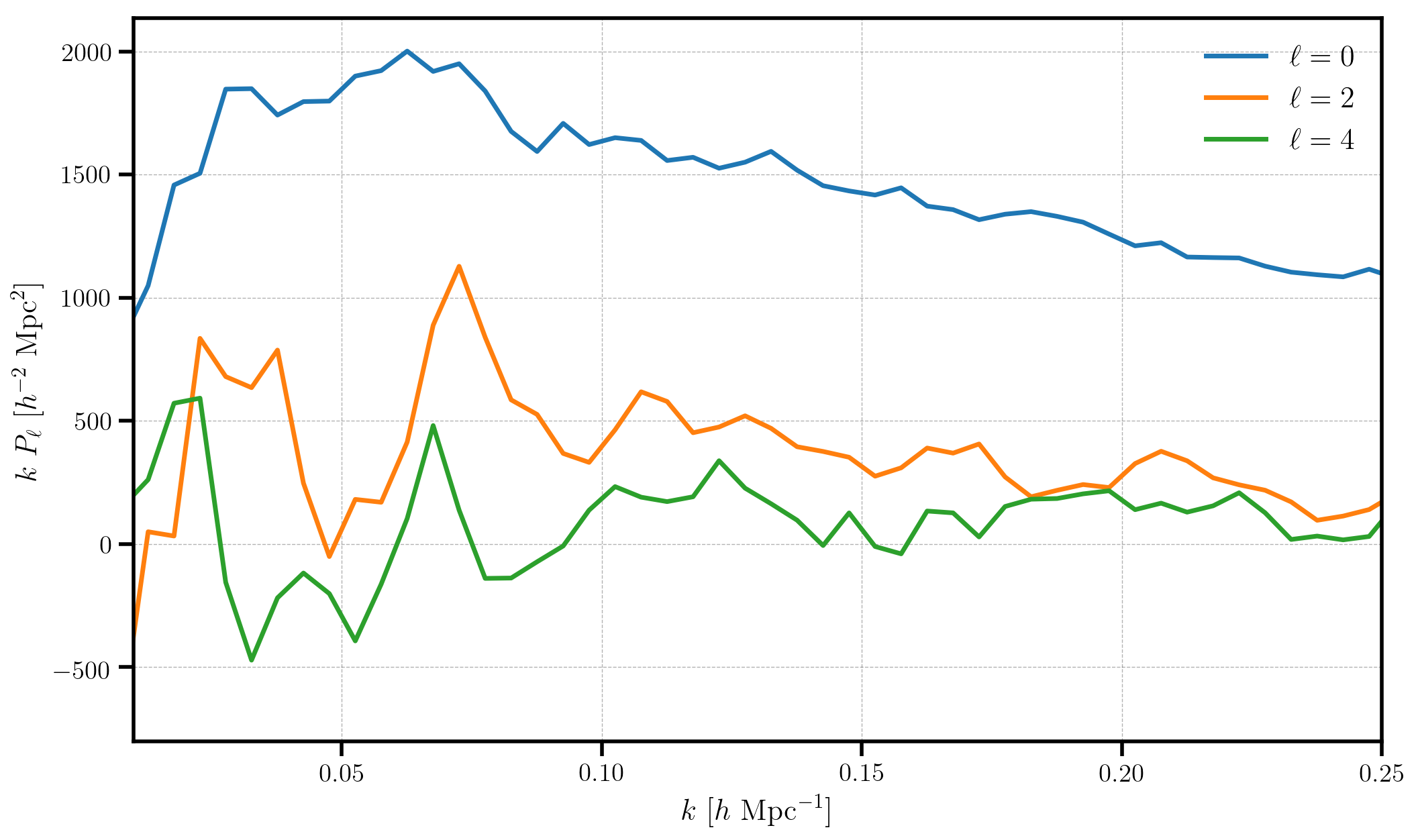
For the LOWZ SGC sample, with \(N = 113525\) objects, the measured multipoles are noiser than for the other DR12 galaxy samples. Nonetheless, we have measured a clear monopole and quadrupole signal, with the hexadecapole remaining largely consistent with zero.
Note that the results here are measured up to the 1D Nyquist frequency,
\(k_\mathrm{max} = k_\mathrm{Nyq} = \pi N_\mathrm{mesh} / L_\mathrm{box}\).
Users can increase the Nyquist frequency and decrease the effects of
aliasing on the measured power by increasing the mesh size. Using
interlacing (by setting interlaced=True) can also reduce the effects
of aliasing on the measured results.
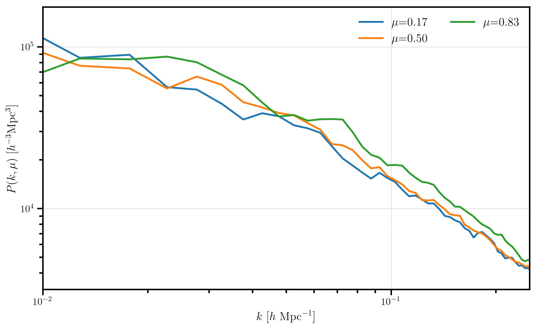
Converting from \(P_\ell(k)\) to \(P(k,\mu)\)
The ConvolvedFFTPower.to_pkmu function allows users to rotate the
measured multipoles, stored as the poles attribute, into
\(P(k,\mu)\) wedges. Below, we convert our measurements of
\(P_0\), \(P_2\), and \(P_4\) into 3 \(\mu\) wedges.
In [15]:
# use the same number of mu wedges and number of multipoles
Nmu = Nell = 3
mu_edges = numpy.linspace(0, 1, Nmu+1)

# get a BinnedStatistic holding the P(k,mu) wedges
Pkmu = r.to_pkmu(mu_edges, 4)
In [16]:
# plot each mu bin
for i in range(Pkmu.shape[1]):
    Pk = Pkmu[:,i] # select the ith mu bin
    label = r'$\mu$=%.2f' % (Pkmu.coords['mu'][i])
    plt.loglog(Pk['k'], Pk['power'].real - Pk.attrs['shotnoise'], label=label)

# format the axes
plt.legend(loc=0, ncol=2)
plt.xlabel(r"$k$ [$h \ \mathrm{Mpc}^{-1}$]")
plt.ylabel(r"$P(k, \mu)$ [$h^{-3}\mathrm{Mpc}^3$]")
plt.xlim(0.01, 0.25)
Out[16]:
(0.01, 0.25)