Log-normal Mocks
In this notebook, we generate a LogNormalCatalog at \(z=0.55\)
using the Planck 2015 cosmology parameters and the Eisenstein-Hu
linear power spectrum fitting formula. We then plot the power spectra in
both real and redshift space and compare to the input linear power
spectrum.
In [1]:
%matplotlib inline
%config InlineBackend.figure_format = 'retina'
In [2]:
from nbodykit.lab import *
from nbodykit import style, setup_logging

import matplotlib.pyplot as plt
plt.style.use(style.notebook)
In [3]:
setup_logging() # turn on logging to screen
Initalizing the Log-normal Mock
Here, we generate a mock catalog of biased objects (\(b_1 = 2\) ) at a redshif \(z=0.55\). We use the Planck 2015 cosmology and the Eisenstein-Hu linear power spectrum fitting formula.
We generate the catalog in a box of side length \(L = 1380 \ \mathrm{Mpc}/h\) with a constant number density \(\bar{n} = 3 \times 10^{-3} \ h^{3} \mathrm{Mpc}^{-3}\).
In [4]:
redshift = 0.55
cosmo = cosmology.Planck15
Plin = cosmology.LinearPower(cosmo, redshift, transfer='EisensteinHu')
b1 = 2.0

cat = LogNormalCatalog(Plin=Plin, nbar=3e-3, BoxSize=1380., Nmesh=256, bias=b1, seed=42)
Real-space Power Spectrum
In this section, we compute and plot the power spectrum, \(P(k,\mu)\), in real space (no redshift distortions) using five \(\mu\) bins.
In [5]:
# convert the catalog to the mesh, with CIC interpolation
real_mesh = cat.to_mesh(compensated=True, window='cic', position='Position')

# compute the 2d P(k,mu) power, with 5 mu bins
r = FFTPower(real_mesh, mode='2d', Nmu=5)
pkmu = r.power
[ 000017.54 ]   0: 10-30 20:51  CatalogMesh     INFO     painted 7887677 out of 7887677 objects to mesh
[ 000017.54 ]   0: 10-30 20:51  CatalogMesh     INFO     mean particles per cell is 0.470142
[ 000017.54 ]   0: 10-30 20:51  CatalogMesh     INFO     sum is 7.88768e+06
[ 000017.55 ]   0: 10-30 20:51  CatalogMesh     INFO     normalized the convention to 1 + delta
[ 000017.91 ]   0: 10-30 20:51  CatalogMesh     INFO     field: (LogNormalCatalog(seed=42, bias=2) as CatalogMesh) painting done
In [6]:
# plot each mu bin
for i in range(pkmu.shape[1]):
    Pk = pkmu[:,i]
    label = r'$\mu$=%.1f' %pkmu.coords['mu'][i]
    plt.loglog(Pk['k'], Pk['power'].real - Pk.attrs['shotnoise'], label=label)

# plot the biased linear power spectrum
k = numpy.logspace(-2, 0, 512)
plt.loglog(k, b1**2 * Plin(k), c='k', label=r'$b_1^2 P_\mathrm{lin}$')

# add a legend and axes labels
plt.legend(loc=0, ncol=2, fontsize=16)
plt.xlabel(r"$k$ [$h \mathrm{Mpc}^{-1}$]")
plt.ylabel(r"$P(k, \mu)$ [$h^{-3} \mathrm{Mpc}^3$]")
plt.xlim(0.01, 0.6)
plt.ylim(500, 2e5)
Out[6]:
(500, 200000.0)
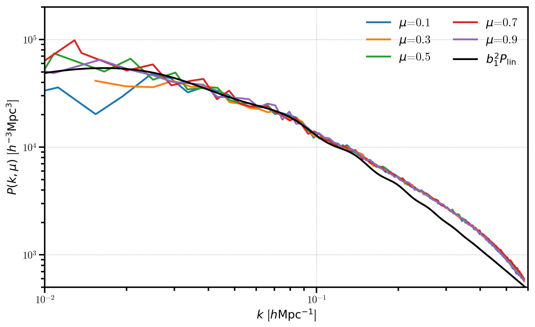
In this figure, we see the power spectrum in real-space is independent of \(\mu\), as expected. At low \(k\), the measured power agrees with the biased linear power \(b_1^2 P_\mathrm{lin}\). But at high \(k\), we see the effects of applying the Zel’dovich approximation to the density field, mirroring the effects of nonlinear evolution.
Redshift-space Power Spectrum
In this section, we compute and plot the power spectrum, \(P(k,\mu)\), in redshift space and see the effects of redshift-space distortions on the 2D power spectrum.
In [7]:
def kaiser_pkmu(k, mu):
    """
    Returns the Kaiser linear P(k,mu) in redshift space

    .. math::

        P(k,mu) = (1 + f/b_1 mu^2)^2 b_1^2 P_\mathrm{lin}(k)
    """
    beta = cosmo.scale_independent_growth_rate(redshift) / b1
    return (1 + beta*mu**2)**2 * b1**2 * Plin(k)
Here, we add redshift space distortions (RSD) along the \(z\)-axis
of the box. We use the VelocityOffset column which is equal to the
Velocity column re-normalized properly for RSD.
In [8]:
LOS = [0,0,1] # the z-axis

# add RSD to the Position
cat['RSDPosition'] = cat['Position'] + cat['VelocityOffset'] * LOS
In [9]:
# from catalog to mesh
rsd_mesh = cat.to_mesh(compensated=True, window='cic', position='RSDPosition')

# compute the 2D power
r = FFTPower(rsd_mesh, mode='2d', Nmu=5, los=LOS)
pkmu = r.power

# plot each mu power bin, normalized by the expected Kaiser power
for i in range(pkmu.shape[1]):
    Pk = pkmu[:,i]
    mu = pkmu.coords['mu'][i]
    label = r'$\mu$=%.1f' %mu

    P = Pk['power'].real-Pk.attrs['shotnoise']
    plt.plot(Pk['k'], P / kaiser_pkmu(Pk['k'], mu), label=label)

# add a legend and axis labels
plt.legend(loc=0, ncol=2)
plt.xlabel(r"$k$ [$h \ \mathrm{Mpc}^{-1}$]")
plt.ylabel(r"$P(k, \mu) / P^\mathrm{Kaiser}(k,\mu)$")
plt.xlim(0.01, 0.6)
plt.ylim(0, 2.5)
[ 000026.10 ]   0: 10-30 20:51  CatalogMesh     INFO     painted 7887677 out of 7887677 objects to mesh
[ 000026.10 ]   0: 10-30 20:51  CatalogMesh     INFO     mean particles per cell is 0.470142
[ 000026.10 ]   0: 10-30 20:51  CatalogMesh     INFO     sum is 7.88768e+06
[ 000026.10 ]   0: 10-30 20:51  CatalogMesh     INFO     normalized the convention to 1 + delta
[ 000026.46 ]   0: 10-30 20:51  CatalogMesh     INFO     field: (LogNormalCatalog(seed=42, bias=2) as CatalogMesh) painting done
/Users/nhand/anaconda/envs/py36/lib/python3.6/site-packages/ipykernel_launcher.py:15: RuntimeWarning: divide by zero encountered in true_divide
  from ipykernel import kernelapp as app
Out[9]:
(0, 2.5)
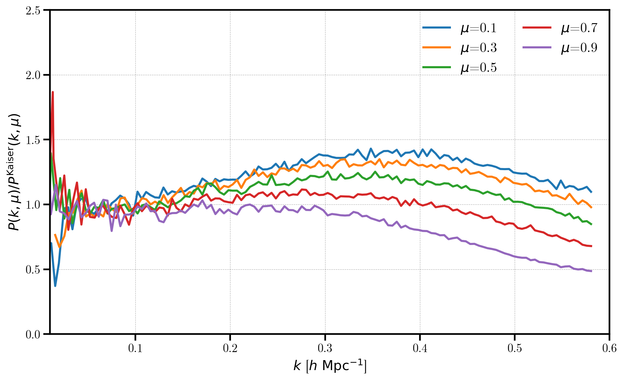
In this figure, we clearly see the effects of RSD, which causes the higher \(\mu\) bins to be damped at high \(k\), relative to the lower \(\mu\) bins. Also, the measured power agrees with the expected Kaiser formula for linear RSD at low \(k\) (where linear theory holds): \(P^\mathrm{Kaiser} = (1 + f/b_1 \mu^2)^2 b_1^2 P_\mathrm{lin}(k)\).